KarpathyLLMChallenge
The content below is generated by LLMs based on the Let’s Reproduce GPT-2 video by Andrej Karpathy
Advanced Model Configuration and Training Optimization
Training large language models like GPT-2 and GPT-3 involves a complex interplay of factors including data preparation, model architecture, training dynamics, and evaluation. This article delves into the advanced techniques and best practices that can significantly enhance the performance and efficiency of training these sophisticated models.
Table of Contents
- Advanced Model Configuration and Training Optimization
- DataLoader and Model Initialization
- Optimization Loop
- Ensuring Efficient Memory Usage
- Leveraging Kernel Fusion with FlashAttention
- Hyperparameter Alignment with GPT Papers
- Hyperparameter Tuning in Line with GPT-3
- Adam Optimizer Configuration
- Explicit Epsilon Value - Gradient Clipping
- Learning Rate Schedule
- Efficient Training with Full Context Windows
- Test Set Contamination Studies
- Performance Metrics and Debugging
- Wrapping Up
- Advanced Learning Rate Scheduling
- Cosine Decay Learning Rate Schedule
- Batch Size Scaling
- Regularization with Weight Decay
- Test Set Contamination Avoidance
- Gradient Clipping
- Training Efficiency with Full Context Windows
- Implementing the Learning Rate Scheduler
- Learning Rate Scheduling in Practice
- Implementing the Learning Rate Scheduler
- Learning Rate Scheduler Visualization
- Model Specific Learning Rates
- Insights into Training GPT-3
- Efficient Sequence Packing
- Further Technical Details
- Terminal and Training Metrics
- Understanding the Learning Rate Scheduler Code
- Training Log Insights
- Dataset Examples
- Training and Debugging
- Diving Deeper into Learning Rate Scheduling
- The Learning Rate Scheduler in Detail
- Key Points to Remember
- Model Training and Optimization
- Insights from the Training Loop
- Tackling Training Data Quality
- Elaborating on GPT-3 Training Details
- Understanding Batch Size Ramp-Up
- Sampling Data Without Replacement
- Implementing Weight Decay
- Training Loop Enhancements
- GPT-3 Training Strategies
- Fine-Tuning the Weight Decay Parameter
- Leveraging Fused AdamW for Performance
- Kernel Fusion Optimization
- Conclusion and Next Steps
- Refining the
configure_optimizersMethod - Performance Improvements with Fused AdamW
- Emphasizing the Importance of Weight Decay Selection
- Learning Rate Scheduling and Optimization
- Advanced Optimizer Configurations
- Evaluation of GPT-3 on NLP Tasks
- Model Size and Learning Rate Adaptations
- Gradient Accumulation: A Solution for Limited Resources
- Implementing Gradient Accumulation in the Training Loop
- Model Architectures Across Different Scales
- Hyperparameters Across Model Sizes
- Conclusion
- Customizing the Learning Rate Schedule
- Optimizer Configuration and Learning Rate Application
- Understanding Gradient Accumulation Mechanism
- The Impact of Reduction on Loss Calculation
- Fine-tuning the Learning Rate Function
- Implementing and Applying the Learning Rate Schedule
- Gradient Accumulation and Loss Normalization
- Real-time Training Metrics Output
- Adjusting Loss Calculation for Gradient Accumulation
- Correcting Gradient Values with Loss Scaling
- Detailed Example of Loss Scaling with Gradient Accumulation
- Implementing a GPT Model Class
- Loss Calculation with Cross Entropy
- Learning Rate Scheduling
- Scaling Loss for Gradient Accumulation
- Detailed Loss Calculation with Gradient Accumulation
- Training Loop with Scaled Loss and Learning Rate Scheduling
- Real-time Performance Metrics
- Accumulating Loss for Gradient Descent
- Understanding Loss Calculation with Gradient Accumulation
- Real-time Training Metrics
- Gradient Scaling and Accumulation
- Real-time Training Metrics and Performance
- Ensuring Accuracy with Batch Size and Gradient Accumulation Steps
- Selecting the Right Device for Training
- Distributed Training with PyTorch
- Monitoring GPU Utilization
- Putting GPUs to Work with Distributed Data Parallel
- Understanding DistributedDataParallel
- Setting Up Distributed Training
- Real-time GPU Monitoring
- Collaborative Gradient Computation
- Initiating Distributed Training
- Detecting Distributed Training Environment
- DataLoader Adjustments for Distributed Training
- Coordinating Distributed Processes
- Master Process in Distributed Training
- Handling Non-DDP Runs
- Initializing the Training Loop
- Distributed Training Configuration
- Handling Device Autodetection
- Gradicum Steps Adjustment
- Model Compilation and Logging
- DataLoader Initialization
- Handling Output in Distributed Systems
- Master Process and Device Autodetection
- Launching Training With Distributed Data Parallel
- DataParallel Configuration
- Training Loop and Device Handling
- Seed Setting and Batch Size Configuration
- Output Management in a Multi-GPU Setup
- DataLoaderLite Example
- Advanced Model Parallelism with DistributedDataParallel
- Final Remarks on DDP Training
- Cleanup Procedures in Distributed Training
- DataParallel Extended Configuration
- DataLoaderLite Implementation
- Advanced DistributedDataParallel Configuration
- Striding Across Processes with DataLoaderLite
- Distributed DataLoader Implementation
- Device and Model Initialization
- Model Compilation and Learning Rate Scheduling
- Parallelism and DistributedDataParallel Configuration
- Setting Up the Training Loop
- Optimizing the Training Process
- Model Compilation and Learning Rate Adjustment
- Distributed Training Efficiency
- Advanced DDP Features
- Synchronizing Across Multiple GPUs
- Backend Initialization and Process Spawning
- Understanding DistributedDataParallel in Depth
- Optimizing Batch Sizes for DDP
- Diving Deeper into the DDP Mechanism
- DataLoader and Training Loop Adjustments for DDP
- Synchronizing Gradients with Gradient Accumulation
- Cautionary Note on DistributedDataParallel
- Detailed Parameters for DistributedDataParallel
- Advanced Gradient Management with DDP
- Disabling Gradient Synchronization
- Communication Hooks in DDP
- Gradient Division by World Size
- Monitoring Training Performance
- Problems and Debugging
- Granular Control of Gradient Synchronization
- Dynamic Gradient Synchronization
- Direct Toggling of Backward Synchronization
- Fine-Tuning the Backward Pass
- Handling Gradient Averaging
- Distributed Averaging of Loss
- Gradient Accumulation and Averaging
- Scaling Loss for Gradient Accumulation
- Synchronization of Gradients
- GPT Neural Network Architecture
- DataLoader Simplification
- Learning Rate Scheduling
- Handling Gradient Accumulation
- Distributed Data Parallel (DDP) Considerations
- Gradient Clipping and Learning Rate Adjustment
- Synchronizing and Measuring Performance
- Learning Rate Scheduler
- Final Debugging and Launching
- Optimizing the Learning Rate Schedule
- Distributed Training Considerations
- Fine-Tuning the Optimization Loop
- Adjusting for DDP Model Configuration
- Configuring Distributed Training
- Adjusting Learning Rate and Model Parameters
- Output During Training - Optimizer Configuration in DDP
- DataLoader and Gradient Accumulation
- Debugging and Problem Solving
- Enhancing the DataLoader for Effective Batching
- Terminal Output for Monitoring Training Progress
- Implementing Gradient Accumulation with
no_sync - Device Auto-detection and DDP Configuration
- Dataset Considerations for GPT-2 and GPT-3 Training
- Deduplication and Data Cleaning
- Dataset Diversity and Quality in LLM Training
- Fine-Tuning Dataset Composition - The Creation of SlimPajama Dataset
- Steps to Enhance Data Quality - Introducing FineWeb Dataset
- FineWeb’s Contributions
- The FineWeb-Edu Subset - Distributed Data Parallel (DDP) Configuration
- Processing Web Data at Scale
- Harnessing Educational Content for LLM Training
- Sampling the FineWeb-Edu Dataset
- Accessing and Utilizing the Data
- Distributed Data Parallel Setup
- Data Processing with Datatrove
- Simplified Data Access and Tokenization
- Filtering Content with LLMs
- Running the Tokenization Script
- Tokenization Process Explained
- Multiprocessing for Efficient Tokenization
- Shard Management
- Tokenization and Sharding Process
- Continued Training Preparation
- Loading Tokens and Initializing Data Loaders
- Managing Shards and Batches
- Configuring the GPT-2 Model
- Initializing the Training Process
- Progress Through Training
- Batch Size and Sequence Length Configuration
- Advanced Training Techniques in GPT Models
- Setting Up the Training Environment
- Learning Rate Scheduling - Calculating Steps for Token Processing
- Quality and Deduplication in Data Preparation
- Model Training Details
- Optimizing the Learning Rate
- Batch Size Configuration
- Device Configuration and Seed Setting
- Distributed Training Setup
- Training Loop Execution
- Launching the Training Script
- Monitoring Training Progress
- Training Metrics
- Batch Size Revisited
- Creating and Configuring the GPT Model
- Learning Rate Schedule
- Training Output Analysis
- Training Considerations
- Enhancing Precision and Model Creation
- Dynamic Learning Rate Adjustment
- Monitoring Training Progress with Live Metrics
- Validating Model on a Validation Set
- Setting up the Device for Training
- Data Loader for Efficient Data Handling
- Model Optimization Configuration
- Model Evaluation and Sampling
- Continuous Validation and Model Saving
- Generating Model Samples During Training
- Printing the Generated Text
- Generated Text Samples
- Examples of Generated Samples
- Training Loop and Sampling Integration
- Sample Generation with Top-K Sampling
- Managing the Random Number Generator (RNG) State
- Continuous Validation and Saving Best Model
- Handling Distributed Training
- Documenting Model Changes and Fixes
- Adjusting the Tokenization Length
- Handling Validation Loss Across Distributed Systems
- Introduction to HellaSwag Evaluation
- HellaSwag’s Sentence Completion Task
- Overview of HellaSwag and Adversarial Filtering
- Evaluating Models with HellaSwag
- Implementation of HellaSwag Evaluation
- HellaSwag Token Completion Methodology
- Implementing HellaSwag Evaluation in Python
- Tracking Model Performance on HellaSwag
- Detailed Evaluation Process
- Continuous Learning and Optimization
- Cross-Entropy Loss in Model Evaluation
- Evaluating Model Predictions
- Performance Metrics
- ElutherAI Harness
- Integrating Periodic Evaluation
- Changes to Training Script
- Debugging Training Issues
- Learning Rate Scheduling
- Logging and Validation
- Sampling from the Model
- Optimization Step
- Fine-Tuning the Optimization Step
- HLSWag Evaluation
- Tracking Correct Predictions
- Synchronizing Statistics Across Processes
- Logging and Sample Generation
- Sample Generation Insights
- Log Directory Setup
- Visualization of Training Progress
- Model Configuration and Initialization
- Training Loop Adjustments
- HellaSwag Evaluation Outcomes
- Considerations on Data Ordering
- Training Data Considerations
- DataLoaderLite Implementation
- Data Ordering and Shuffling
- Training Batch Size Configuration
- Learning Efficiency Insights
- Considerations for Hyperparameters Adjustment
- Setting Up the Training Environment
- Visualization of Extended Training Results
- Sequence Length Adjustment for Model Training
- Loss Metrics and Comparison with Other Models
- DataLoaderLite and Training Process
- Model Creation and Configuration
- Sample Generation Insights
- Validation Loss Evaluation
- Master Process Validation Loss Reporting
- Visualization of Training and Evaluation Metrics
- Checkpointing and State Management
- Enhanced Evaluation with Luther
- Language Model Evaluation Harness
- Comparison With Other Models
- Pre-training and Fine-tuning
- Continuing Pre-training and Checkpointing
- Exploring Alternative Implementations
- LN.C: A High-Performance C-CUDA Implementation
- Training GPT2 in LN.C
- Side-by-Side Comparison
- Observations and Performance
- LN.C vs. PyTorch: Performance and Space Efficiency
- Command-Line Training with PyTorch
- LN.C: A Parallel Implementation
- LLM.C: Simple and Pure C/CUDA Language Models
- Quick Start for LLM.C
- Training Insights and Tokenization
- Consistency Between Implementations
- Visualizing Model Training and Tokenization
- Addressing Training Anomalies and Optimization
- Building and Understanding nanoGPT
- Community Engagement and Contributions
- Causal Self-Attention in GPT-2 Training
- Reflecting on Progress and Future Directions
Advanced Model Configuration and Training Optimization
As we progress with the implementation of our GPT-2 model, it’s essential to optimize the training process to utilize our hardware efficiently and align with the best practices outlined in the GPT-2 and GPT-3 papers. Let’s delve into the configuration of our train_gpt2.py script, making key adjustments for performance gains.
DataLoader and Model Initialization
To start, we initialize our data loader with a batch size (B) of 16 and a maximum sequence length (T) of 1024 tokens:
train_loader = DataLoader(list(B=16, T=1024))
Next, we set the matrix multiplication precision for floating-point operations to high, which is crucial for maintaining model accuracy during training:
torch.set_float32_matmul_precision('high')
We then initialize the GPT model configuration with an adjusted vocabulary size to a more hardware-friendly number, ensuring more efficient computation:
# Adjust vocabulary size for optimization
model = GPT(GPTConfig(vocab_size=53004))
model.to(device)
model = torch.compile(model)
Optimization Loop
With our model and data loader set up, we proceed to the optimization loop. We use the AdamW optimizer with a learning rate of 3e-4, which is a commonly used optimizer for training language models due to its effectiveness in handling sparse gradients:
optimizer = torch.optim.AdamW(model.parameters(), lr=3e-4)
During the training loop, we ensure that each batch of data is processed and optimized efficiently:
for i in range(50):
    t0 = time.time()
    x, y = train_loader.next_batch()
    x, y = x.to(device), y.to(device)
    optimizer.zero_grad()

    # Enable mixed precision training for performance optimization
    with torch.autocast(mode='x', device_type=torch.bfloat16):
        logits, loss = model(x, y)

    loss.backward()
    optimizer.step()
    torch.cuda.synchronize() # wait for the GPU to finish work
    t1 = time.time()

    # Calculate tokens processed per second for performance measurement
    dt = t1 - t0 # time difference in seconds
    tokens_processed = train_loader.B * train_loader.T
    tokens_per_sec = tokens_processed / dt
    print(f"Step: {i}, Loss: {loss.item()}, Tokens/sec: {tokens_per_sec}")
In this loop, we employ mixed precision training using PyTorch’s autocast to enhance training speed without compromising the model’s performance. The torch.cuda.synchronize() function ensures that we accurately measure the time taken per iteration by waiting for the GPU to complete its work.
Ensuring Efficient Memory Usage
One key aspect of optimization involves ensuring that tensors and operations are aligned with the GPU’s architecture, which favors powers of two. By adjusting the vocabulary size to 53004—a number with many factors of two—we can reduce the need for special case handling in CUDA kernels, leading to improved training speed:
# Adjusting vocabulary size to a more hardware-friendly number
vocab_size = 53004
This seemingly minor change can lead to significant performance gains due to better utilization of the GPU’s memory bandwidth and compute capabilities.
Leveraging Kernel Fusion with FlashAttention
Another sophisticated optimization is the use of FlashAttention, an algorithmic improvement that fuses multiple operations into a single kernel, drastically reducing memory bandwidth usage. By replacing multiple lines of attention calculation with FlashAttention, we can further accelerate our training loop:
# Replace attention mechanism with FlashAttention for improved performance
with torch.autocast(mode='x', device_type=torch.bfloat16):
    logits, loss = model.flash_attention(x, y)
Hyperparameter Alignment with GPT Papers
Finally, we align our training hyperparameters with the guidelines provided in the GPT-2 and GPT-3 papers. While the GPT-2 paper is vague about the specifics of the training setup, the GPT-3 paper’s appendix offers a more detailed list of hyperparameters used for training. We incorporate these recommendations into our training script to ensure we’re following the best practices that led to the success of these models.
In sum, by carefully configuring our data loader, optimizing tensor sizes, employing mixed precision training, leveraging kernel fusion, and adhering to the hyperparameters outlined in seminal papers, we can significantly enhance the performance and efficiency of our GPT-2 model training. These advanced optimizations are crucial for handling the computational demands of large language models and achieving state-of-the-art results.
Hyperparameter Tuning in Line with GPT-3
In our quest to replicate the architecture and success of GPT models, it becomes evident that the devil is in the details—especially when it comes to hyperparameter tuning. The GPT-3 paper provides a plethora of subtle but critical details that ultimately make a significant impact on the model’s performance.
Adam Optimizer Configuration
For fine-tuning our model’s training process, we’ll adhere closely to the configurations recommended in the GPT-3 paper. This involves setting the optimizer parameters to specific values that have been empirically proven to work well for such large models.
Let’s configure our optimizer with the recommended beta values:
# Configure optimizer with GPT-3 recommended hyperparameters
optimizer = torch.optim.AdamW(model.parameters(), lr=3e-4, betas=(0.9, 0.95), eps=1e-8)
These beta values control the exponential decay rates for the moment estimates in Adam, which in turn affect the step sizes taken during optimization.
Explicit Epsilon Value
With large-scale models, even the smallest parameters—such as epsilon—can have a significant impact. The GPT-3 paper specifies an epsilon value of 1e-8. Including this value explicitly ensures that we’re fully aligned with their setup:
# Explicitly define epsilon value as per GPT-3 recommendations
optimizer = torch.optim.AdamW(model.parameters(), lr=3e-4, betas=(0.9, 0.95), eps=1e-8)
Gradient Clipping
Gradient clipping is a technique used to prevent exploding gradients in neural networks, which is even more important in the context of such large models as GPT-3. The GPT-3 paper suggests clipping the gradient norm at 1.0 to stabilize training:
# Clip gradients during training to prevent exploding gradients
for i in range(50):
    ...
    loss.backward()
    torch.nn.utils.clip_grad_norm_(model.parameters(), max_norm=1.0)
    optimizer.step()
    ...
The function torch.nn.utils.clip_grad_norm_ modifies gradients in place and ensures that the norm of the parameter gradients does not exceed 1.0.
Learning Rate Schedule
GPT-3 introduces a sophisticated learning rate schedule that involves a warmup period followed by a cosine decay. To implement this, we would need to adjust the learning rate over time:
# Example of learning rate scheduler setup (requires further implementation)
scheduler = torch.optim.lr_scheduler.CosineAnnealingLR(optimizer, T_max=260e9, eta_min=lr*0.1)
This scheduler requires additional logic to handle the warmup phase and adjust T_max and eta_min based on the number of tokens processed.
Efficient Training with Full Context Windows
To train more efficiently, the GPT-3 paper suggests always training on sequences with the full context window size. This means packing multiple documents into a single sequence when they are shorter than the maximum context length, which increases computational efficiency:
# Pack multiple documents into a single sequence for efficient training
train_sequences = pack_documents(train_data, max_context_size=2048)
The above pseudo-code implies that you would need a function like pack_documents to handle this operation. The GPT-3 model uses a special end-of-text token to separate documents within a sequence.
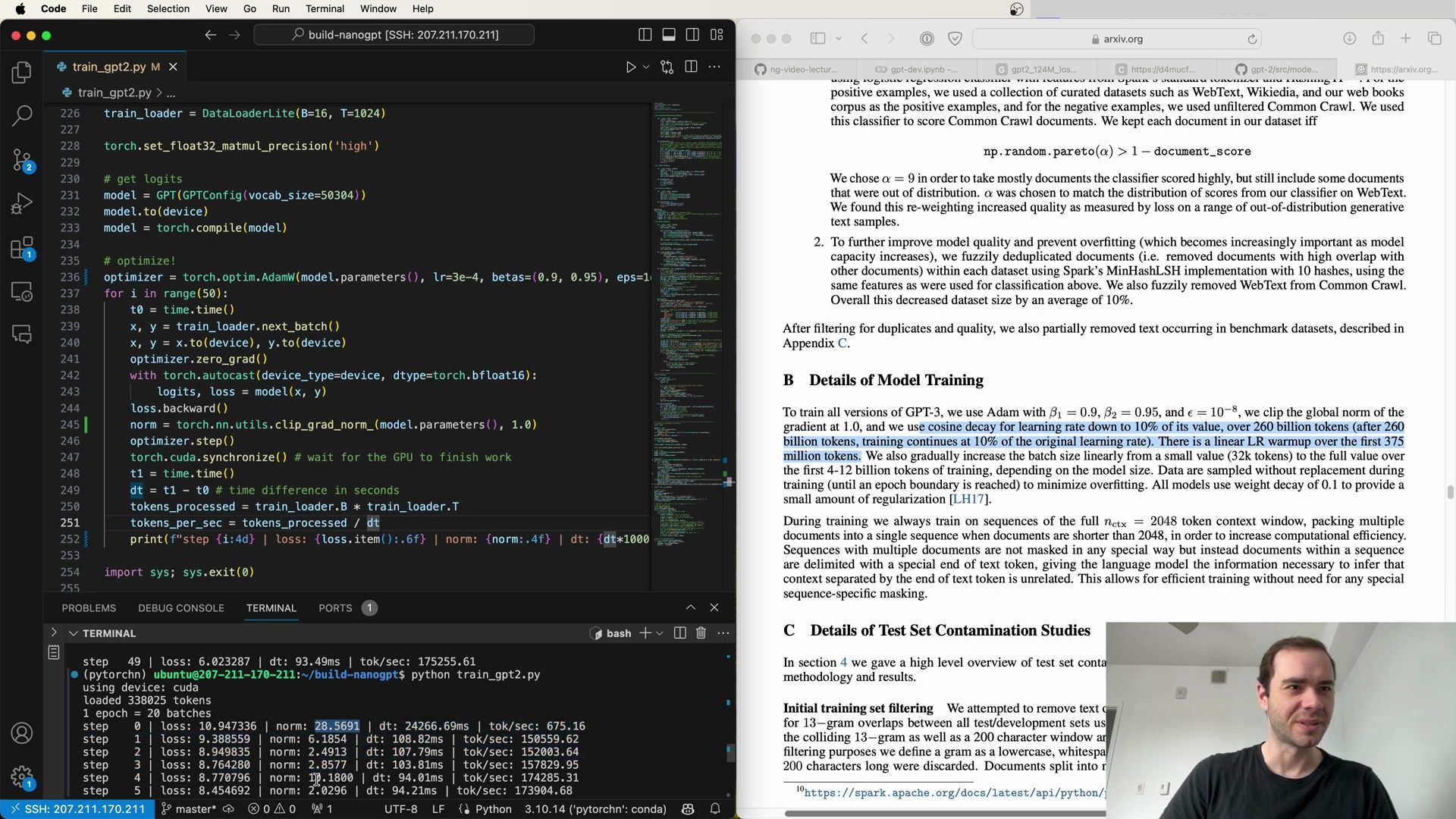
Test Set Contamination Studies
Moreover, the GPT-3 paper details their methodology to minimize test set contamination. They filter out training data that overlaps with test and development sets by searching for 13-gram overlaps and discarding any colliding sequences:
# Filter training set for test set contamination
filtered_train_data = filter_contamination(train_data, test_sets, n_gram=13)
Implementing such a filter function would involve defining what constitutes an overlap and how to handle the surrounding context of the identified overlap.
Performance Metrics and Debugging
During training, it is crucial to keep an eye on various performance metrics. One such metric is the norm of the gradient, which can provide insights into the training stability:
# Print out the norm of the gradient to monitor training stability
for i in range(50):
    ...
    norm = torch.nn.utils.clip_grad_norm_(model.parameters(), max_norm=1.0)
    print(f"Step: {i}, Loss: {loss.item()}, Gradient Norm: {norm}, Tokens/sec: {tokens_per_sec}")
Monitoring the gradient norm allows us to detect issues early on. A well-behaved norm indicates stable training, while a climbing norm may signal that the model is destabilizing.
Wrapping Up
By meticulously aligning our model’s hyperparameters with those detailed in the GPT-3 paper, employing gradient clipping, and monitoring performance metrics, we set the stage for training a language model that could potentially rival the performance of GPT-3. While we may not have access to the weights of GPT-3, these practices bring us closer to the frontier of language modeling.
In the next section, we’ll explore additional strategies to further enhance our model’s training process, including data sampling techniques and model regularization. Stay tuned as we continue to delve deeper into the intricacies of training state-of-the-art language models.
Advanced Learning Rate Scheduling
In the journey to replicate the performance of GPT-3, an advanced learning rate scheduling is used. This is not a fixed learning rate as one might typically see but involves a warmup phase followed by a cosine decay. This sophisticated scheduling was meticulously detailed in the GPT-3 paper and is essential to achieving optimal results.
Cosine Decay Learning Rate Schedule
GPT-3 employs a learning rate schedule that starts with a linear warmup period. After this, it transitions to a cosine decay that reduces the learning rate to 10% of its initial value over a vast span of 260 billion tokens. This is followed by continued training at this reduced rate.
Here’s how we can implement this in PyTorch:
import math
import torch

# Configuration parameters for the scheduler
max_lr = 3e-4
min_lr = max_lr * 0.1
warmup_steps = 375e6  # 375 million tokens
total_steps = 260e9   # 260 billion tokens
current_step = 0

# Function to calculate learning rate
def get_lr(current_step):
  if current_step < warmup_steps:
    # Linear warmup
    return max_lr * (current_step + 1) / warmup_steps
  else:
    # Cosine decay to 10% of the max_lr
    decay_steps = current_step - warmup_steps
    decay_ratio = decay_steps / (total_steps - warmup_steps)
    cos_decay = (1.0 + math.cos(math.pi * decay_ratio)) / 2
    return min_lr + (max_lr - min_lr) * cos_decay

# Update learning rate at each training step
for step in range(int(total_steps)):
  lr = get_lr(step)
  for param_group in optimizer.param_groups:
    param_group['lr'] = lr
It is important to note that the learning rate scheduling is a critical component of GPT-3’s training success, providing a controlled adjustment of the learning rate that promotes better convergence over time.
Batch Size Scaling
To further refine our training process, it is also recommended to scale up the batch size linearly. This gradual increase happens over the first 4 to 12 billion tokens of training, depending on the model size. Increasing the batch size over time allows the model to start learning from a more manageable amount of data and then leverage more significant amounts of data for learning as the training progresses.
Regularization with Weight Decay
GPT-3 introduces a small amount of regularization through weight decay. This strategy is designed to prevent overfitting by adding a penalty for larger weights in the model. In PyTorch, this can be achieved by setting the weight_decay parameter in the optimizer:
optimizer = torch.optim.AdamW(model.parameters(), lr=3e-4, betas=(0.9, 0.95), eps=1e-8, weight_decay=0.1)
This addition of weight decay acts as a form of L2 regularization, encouraging the model to find simpler patterns within the data, which can generalize better to new, unseen data.
Test Set Contamination Avoidance
An often overlooked but crucial aspect of training large language models is avoiding contamination between training and test datasets. For GPT-3, a meticulous process was used to ensure that the training data did not include any sequences that overlapped with the test or development sets.
This was accomplished by searching for 13-gram overlaps and removing not just the overlapping sequence but also a substantial context around it. If a document was split into multiple parts due to this filtering process and the resulting pieces were too short, they were discarded. This approach is highly important to ensure that the model’s performance is a true reflection of its ability to generalize and not merely a result of memorizing parts of the test set.
Gradient Clipping
Another critical aspect of stable training is gradient clipping, which we’ve already touched upon earlier. It’s worth reiterating its importance as an effective technique to prevent the exploding gradients problem, which is particularly prevalent in large models like GPT-3. With each training step, we clip the gradient norm at 1.0 to stabilize the training:
# Perform gradient clipping
for i in range(max_training_steps):
    ...
    loss.backward()
    norm = torch.nn.utils.clip_grad_norm_(model.parameters(), 1.0)
    optimizer.step()
    ...
The gradient norm values during the initial stages of training can be quite high due to the model parameters being randomly initialized. However, as training progresses, the norm typically stabilizes. Sudden spikes or deviations from this pattern can be an indicator of issues in the training process and should be investigated.
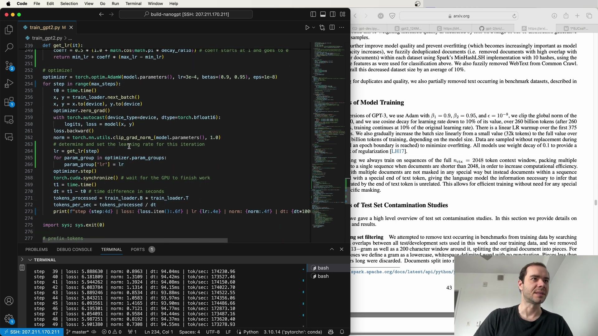
Training Efficiency with Full Context Windows
In order to maximize computational efficiency during training, GPT-3 always utilizes sequences with the full context window of 2048 tokens. This is done by packing multiple documents into a single sequence when they are shorter than the context size. No special masking is necessary for these sequences, as documents are separated by a special end-of-text token, allowing the model to distinguish unrelated contexts within the same sequence.
Implementing the Learning Rate Scheduler
To implement the aforementioned learning rate schedule with warmup and cosine decay, we can use the following code snippet:
# Set precision for matrix multiplication
torch.set_float32_matmul_precision('high')

# Initialize the model
model = GPT(GPTConfig(vocab_size=50304))
model.to(device)
model = torch.compile(model)

# Learning rate scheduling parameters
max_lr = 3e-4
min_lr = max_lr * 0.1
warmup_steps = 375e6
total_steps = 260e9

# Define the learning rate schedule function
def get_lr(i):
    if i < warmup_steps:
        return max_lr * (i + 1) / warmup_steps
    if i > total_steps:
        return min_lr
    decay_ratio = (i - warmup_steps) / (total_steps - warmup_steps)
    coeff = (1.0 + math.cos(math.pi * decay_ratio)) / 2
    return min_lr + coeff * (max_lr - min_lr)

# Initialize the optimizer
optimizer = torch.optim.AdamW(model.parameters(), lr=3e-4, betas=(0.9, 0.95), eps=1e-8)

# Apply the learning rate schedule during optimization
for step in range(int(total_steps)):
    lr = get_lr(step)
    for param_group in optimizer.param_groups:
        param_group['lr'] = lr
    # Proceed with training steps
By adhering to these detailed training strategies, including the learning rate schedule, batch size scaling, regularization techniques, and avoidance of test set contamination, we approach the frontier of training large-scale language models. These practices are instrumental in refining the model to achieve performance on par with groundbreaking models such as GPT-3.
Learning Rate Scheduling in Practice
In the context of training models like GPT-3, the learning rate typically starts close to zero, ramps up linearly during a warmup phase, and then decays following a cosine curve to a predefined minimum. While the minimum learning rate in some settings might be zero, in the case of GPT-3, the team used a non-zero minimum as part of their cosine decay strategy.
The learning rate schedule is pivotal, affecting the model’s ability to converge to a suitable set of weights. During training, the learning rate is gradually decreased, following a cosine function, down to 10% of its maximum value over a significant amount of steps, and then training continues at this reduced rate.
Implementing the Learning Rate Scheduler
To implement this type of learning rate schedule in PyTorch, we can utilize the following code, which includes a linear warmup followed by a cosine decay:
import math
import time
import torch

# Set precision for matrix multiplication
torch.set_float32_matmul_precision('high')

# Initialize the model
model = GPT(GPTConfig(vocab_size=50304))
model.to(device)
model = torch.compile(model)

# Learning rate scheduling parameters
max_lr = 3e-4
min_lr = max_lr * 0.1
warmup_steps = 10
max_steps = 50

# Define the learning rate schedule function
def get_lr(step):
    if step < warmup_steps:
        # 1) Linear warmup for warmup_steps
        return max_lr * (step + 1) / warmup_steps
    if step >= max_steps:
        # 2) After max_steps, use the minimum learning rate
        return min_lr
    # 3) Cosine decay down to min_lr in between
    decay_ratio = (step - warmup_steps) / (max_steps - warmup_steps)
    assert 0 <= decay_ratio <= 1
    coeff = 0.5 * (1.0 + math.cos(math.pi * decay_ratio))
    return min_lr + coeff * (max_lr - min_lr)

# Initialize optimizer
optimizer = torch.optim.AdamW(model.parameters(), lr=3e-4, betas=(0.9, 0.95), eps=1e-8)

# Training loop with learning rate scheduling
for step in range(max_steps):
    t0 = time.time()
    X, y = train_loader.next_batch()
    X, y = X.to(device), y.to(device)

    optimizer.zero_grad()
    logits = model(X)
    loss = loss_fn(logits, y)
    loss.backward()
    optimizer.step()

    t1 = time.time()

    # Print training metrics
    print(f'Step: {step}, Loss: {loss.item()}, Time/step: {t1-t0}, tok/sec: {tokens_per_second}')
This code snippet begins with a linear increase of the learning rate during the warmup phase and then transitions to a cosine decay, where the learning rate gradually decreases to a minimum value, emulating the schedule used in GPT-3’s training.
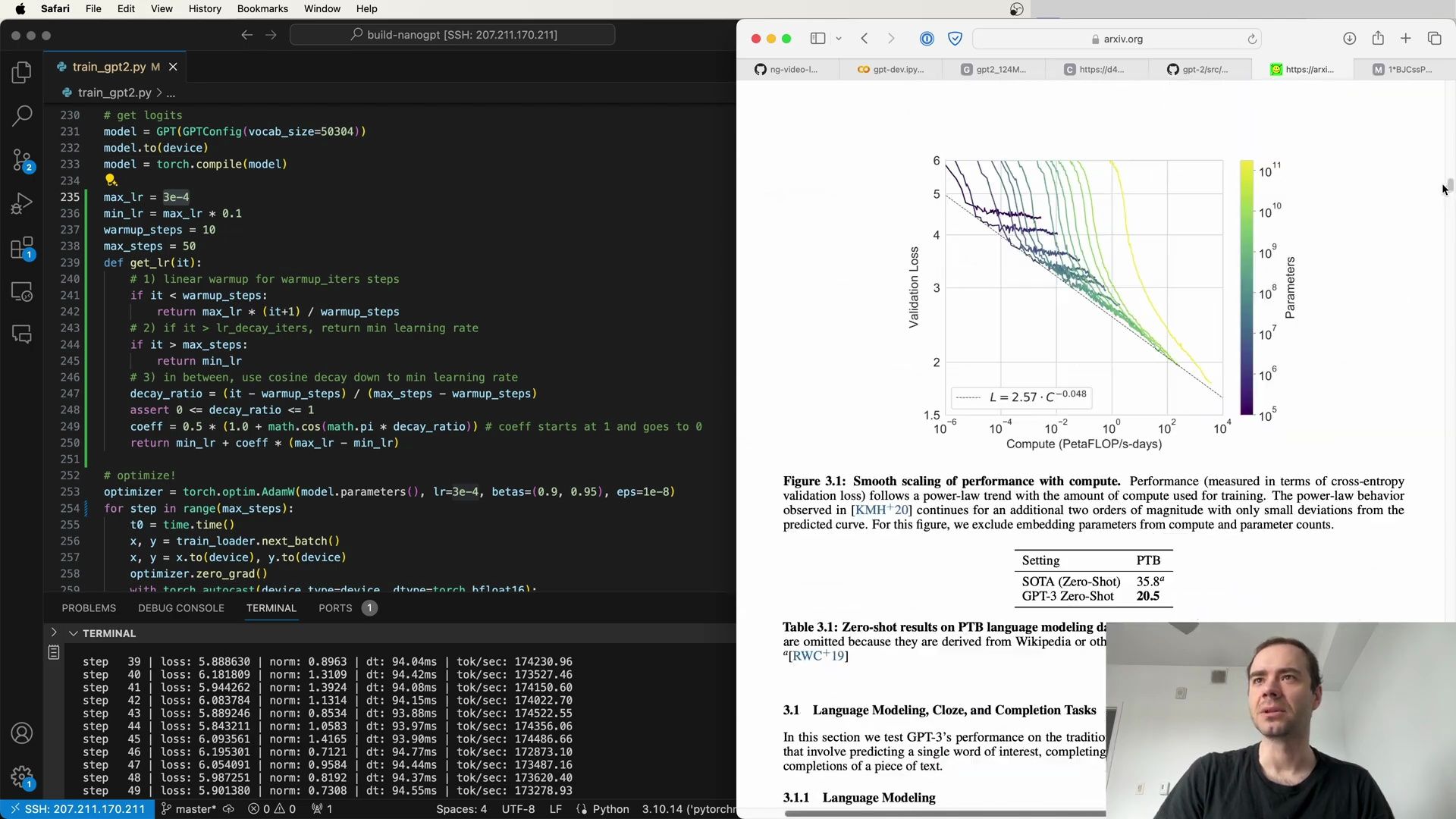
Learning Rate Scheduler Visualization
To better understand the effects of this learning rate schedule, let’s visualize it:
In the graph above, you can see the linear ramp-up during the warmup phase followed by the cosine decay. The visualization helps to intuitively grasp how the learning rate evolves over time, which is critical for the convergence of large models like GPT-3.
Model Specific Learning Rates
It’s important to note that the optimal maximum learning rate might vary depending on the model size. In the case of GPT-3, different configurations of the model used different learning rates:
- GPT-3 Small:
6.0 x 10^-4 - GPT-3 Medium:
3.0 x 10^-4 - GPT-3 Large:
2.5 x 10^-4 - GPT-3 XL:
2.0 x 10^-4 - And so on…
Each model configuration requires its own learning rate to optimize performance, as indicated in the partially visible table:
The learning rates for each model size are carefully chosen based on empirical results and are essential for training stability and efficiency.
Insights into Training GPT-3
The training process for all versions of GPT-3 includes several vital components, as extracted from the script and screenshot descriptions:
- Adam Optimizer: The use of the Adam optimizer with hyperparameters
β1 = 0.9,β2 = 0.95, andε = 1e-8. - Gradient Clipping: Clipping the global norm of the gradient at
1.0to prevent gradients from exploding. - Cosine Decay: Employing cosine decay for the learning rate down to
10%of its initial value over an extensive number of tokens. - Batch Size Scaling: Increasing the batch size linearly from a small initial value to the full value over billions of tokens, depending on the model size.
- Regularization: Implementing weight decay of
0.1as a form of L1 regularization.
The models were trained for a total of 300 billion tokens, emphasizing the massive scale of the data processed.
Efficient Sequence Packing
To increase computational efficiency, sequences are packed with the full context window of 2048 tokens. Shorter documents are concatenated with longer ones, separated by a special end-of-text token, which signals the model that the contexts are not related:
# Sample Python code illustrating the concept:
sequences = []
for doc in documents:
    if len(doc) < context_window:
        sequences.append(doc + end_of_text_token)
    else:
        sequences.append(doc)
This approach allows multiple documents to be processed in a single sequence without the need for special masking, thus optimizing the use of computational resources.
Further Technical Details
An excerpt from the technical details reveals additional insights into the training regimen and the measures taken to prevent test set contamination:
-
Test Set Contamination Avoidance: Efforts were made to ensure that the training data was free from overlaps with the test and development sets. Any overlaps and a surrounding context window were removed, with too-short resulting documents being discarded.
-
Model Architectures: The models follow the same architecture as GPT-2, including pre-normalization and tokenization strategies, with variations in the size and parameters to explore the effects of scale.
Terminal and Training Metrics
The training process is often accompanied by a live feed of metrics in the terminal, providing real-time updates on the progress. These metrics typically include the number of tokens processed per second, loss values, and time taken per training step.
Such metrics are crucial for monitoring the model’s learning and ensuring that the training is proceeding as expected. This real-time feedback loop is an indispensable part of the training workflow for large models like GPT-3.
Understanding the Learning Rate Scheduler Code
In optimizing our model’s performance, we pay special attention to the learning rate as it crucially influences the model’s ability to converge to a good set of parameters. The learning rate scheduler plays a pivotal role in this process, and the code provided gives us an in-depth look at its implementation. Let’s dissect the provided Python code to understand each component:
# Learning rate schedule parameters
max_lr = 6e-4  # The maximum learning rate
min_lr = max_lr * 0.1  # The minimum learning rate (10% of max_lr)
warmup_steps = 10  # The number of steps over which the learning rate is warmed up
max_steps = 50  # The maximum number of steps

# The learning rate scheduling function
def get_lr(step):
    if step < warmup_steps:
        # Warm-up region: linearly increase the learning rate
        return max_lr * (step + 1) / warmup_steps
    if step >= max_steps:
        # After max_steps, use the minimum learning rate
        return min_lr
    # In between: use cosine decay down to the minimum learning rate
    decay_ratio = (step - warmup_steps) / (max_steps - warmup_steps)
    assert 0 <= decay_ratio <= 1
    coeff = 0.5 * (1.0 + math.cos(math.pi * decay_ratio))
    return min_lr + coeff * (max_lr - min_lr)

# Optimizing with the AdamW optimizer
optimizer = torch.optim.AdamW(model.parameters(), lr=3e-4, betas=(0.9, 0.95), eps=1e-8)

# Training loop
for step in range(max_steps):
    t0 = time.time()
    x, y = train_loader.next_batch()
    x, y = x.to(device), y.to(device)
    optimizer.zero_grad()
    with torch.autocast(device_type=device, dtype=torch.bfloat16):
        logits, loss = model(x, y)
    loss.backward()
    optimizer.step()
    t1 = time.time()

    # Log training metrics
    print(f'Step: {step}, Loss: {loss.item()}, Time/step: {t1-t0}, tok/sec: {tokens_per_second}')
In this code snippet, we start with a linear warmup of the learning rate, followed by a cosine decay. The learning rate increases linearly from zero (to avoid a non-useful learning rate of zero) to the maximum learning rate (max_lr), then it decays following a cosine curve down to the minimum learning rate (min_lr), which is 10% of the maximum learning rate.
Key Elements in the Learning Rate Scheduler Code:
- Linear Warmup: The learning rate starts very low and linearly increases during the warmup phase to the maximum learning rate, avoiding the pitfall of a zero learning rate.
- Cosine Decay: After the warmup phase, the learning rate follows a cosine decay pattern, which gradually decreases it to the minimum learning rate.
- AdamW Optimizer: The AdamW optimizer is used with specific hyperparameters
betas=(0.9, 0.95)andeps=1e-8. - Mixed Precision Training: The
torch.autocastcontext manager is used for mixed-precision training, which allows for faster computation and reduced memory usage.
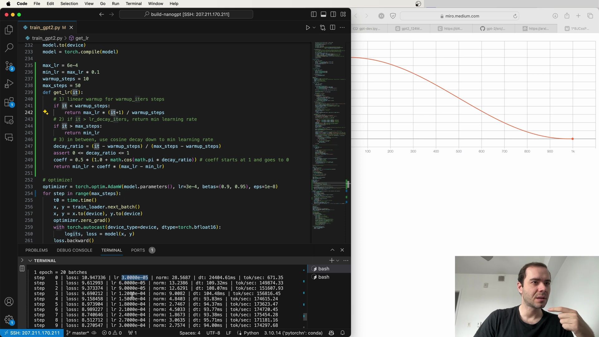
Training Log Insights
During training, it’s essential to monitor the model’s performance through logs that provide insights into loss, learning rate, and tokens processed per second. Below is an example of the training log output:
step    | loss: 5.8868630   | lr: 0.0006   | dt: 94.20ms | tok/sec: 174320.96
step    | loss: 5.8488910   | lr: 0.0006   | dt: 94.20ms | tok/sec: 174320.96
...
From these logs, we can extract the following details:
- Step: The current step number in the training process.
- Loss: The loss value at the current step, which we aim to minimize.
- Learning Rate (lr): The learning rate applied at the current step, adjusted according to the schedule.
- Time per Step (dt): The duration in milliseconds it takes to complete one training step.
- Tokens per Second (tok/sec): The number of tokens processed per second.
By monitoring these metrics, we can gauge the efficiency and effectiveness of the training process.
Dataset Examples
The training data plays a significant role in how the model learns to perform tasks. Here are examples of the formatted datasets for PIQA and COPA, respectively:
- PIQA Example:
- Context: How to apply sealant to wood.
- Correct Answer: Using a brush, brush on sealant onto wood until it is fully saturated with the sealant.
- Incorrect Answer: Using a brush, drip on sealant onto wood until it is fully saturated with the sealant.
- COPA Example:
- Context: (CNN) Yuval Rabin, whose father, Yitzhak Rabin, was assassinated while serving as Prime Minister of Israel, criticized Donald Trump for appealing to ‘Second Amendment people’ in a speech and warned that the words that politicians use can incite violence and undermine democracy.
- Correct Answer: Referencing his father, who was shot and killed by an extremist amid political tension in Israel in 1995, Rabin condemned Donald Trump’s aggressive rhetoric.
- Incorrect Answer: Referencing his father, who was shot and killed by an extremist amid political tension in Israel in 1995, Rabin condemned Donald Trump’s aggressive rhetoric.
These examples illustrate how the datasets are structured, with contexts provided along with correct and incorrect answers, which helps the model learn to distinguish between the two.
Training and Debugging
As we train our model, it is not uncommon to encounter issues that require debugging. The training logs are invaluable in this regard, offering real-time feedback on the model’s performance and any potential issues. Debugging may involve examining the loss, gradients, or tokens per second to ensure that the training is progressing as expected.
In the screenshot, we observe a debug console with various metrics that provide insight into the training process. The console includes information such as the current step, loss, learning rate, and tokens processed per second, all of which are critical for diagnosing and resolving issues during training.
By carefully examining training logs and employing debugging tools, we can ensure that our model is learning effectively and make any necessary adjustments to the training regimen.
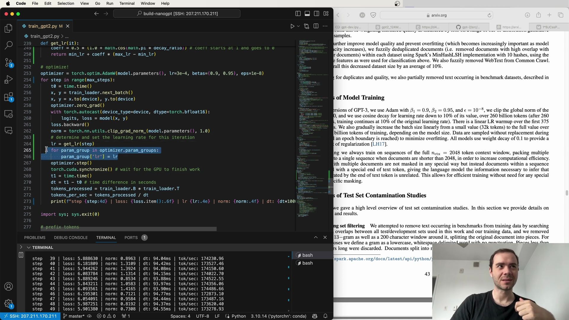
Diving Deeper into Learning Rate Scheduling
In the pursuit of fine-tuning our model’s training process, we delve into the nuances of learning rate scheduling, an area that has been popularized and extended significantly in recent research. The learning rate scheduler we’re exploring is inspired by the methods used in training GPT-2 and GPT-3, although with some modifications tailored to our specific needs.
The Learning Rate Scheduler in Detail
The scheduler’s code is a critical component of our training strategy. Below is a breakdown of the code block that defines the learning rate scheduler:
# Learning rate schedule parameters
max_lr = 6e-4  # The maximum learning rate
min_lr = max_lr * 0.1  # The minimum learning rate (10% of max_lr)
warmup_steps = 10  # The number of steps over which the learning rate is warmed up
max_steps = 50  # The maximum number of steps

# Learning rate scheduling function
def get_lr(t):
    # Linear warmup for warmup_iters steps
    if t < warmup_steps:
        return max_lr * (t+1) / warmup_steps
    # Cosine decay down to min learning rate
    decay_ratio = (t - warmup_steps) / (max_steps - warmup_steps)
    coeff = 0.5 * (1.0 + math.cos(math.pi * decay_ratio))  # coeff starts at 1 and goes to 0
    assert 0 <= decay_ratio <= 1
    return min_lr + coeff * (max_lr - min_lr)

# Optimizer instantiation using AdamW
optimizer = torch.optim.AdamW(model.parameters(), lr=3e-4, betas=(0.9, 0.95), eps=1e-8)

# Training loop for updating model parameters
for step in range(max_steps):
    # ... training code ...
Key Points to Remember
- Warmup Period: The learning rate starts very low and increases linearly during the warmup phase to the maximum learning rate.
- Cosine Decay: Following the warmup, the learning rate decreases following a cosine curve to the minimum learning rate.
- Parameters: The
max_lr,min_lr,warmup_steps, andmax_stepsparameters can be adjusted to suit the model’s training needs.
Model Training and Optimization
The training process is at the heart of developing a robust and effective model. Let’s take a closer look at the training loop, where the learning rate scheduling function and the optimizer come into play:
# Training loop
for step in range(max_steps):
    # Record the time at the start of the step
    t0 = time.time()
    # Obtain the next batch of training data
    x, y = train_loader.next_batch()
    # Move the batch to the appropriate device (e.g., GPU)
    x, y = x.to(device), y.to(device)
    # Prepare the model for a new gradient calculation
    optimizer.zero_grad()
    # Forward pass through the model with autocasting to mixed precision
    with torch.autocast(device_type=device, dtype=torch.bfloat16):
        logits, loss = model(x, y)
    # Backward pass to compute the gradient
    loss.backward()
    # Clip gradients to prevent exploding gradient problem
    norm = torch.nn.utils.clip_grad_norm_(model.parameters(), 1.0)
    # Update the learning rate based on the current step
    lr = get_lr(step)
    for param_group in optimizer.param_groups:
        param_group['lr'] = lr
    # Update model parameters
    optimizer.step()
    # Synchronize GPU to ensure all tasks are completed before moving on
    torch.cuda.synchronize()
    # Record the time at the end of the step
    t1 = time.time() - t0
Insights from the Training Loop
- Gradient Clipping: To prevent the notorious exploding gradient problem, gradients are clipped to a norm of 1.0.
- Learning Rate Updates: The learning rate for each step is determined by the
get_lrfunction and dynamically updated. - Mixed Precision Training: The
torch.autocastcontext manager is used to enable mixed precision, thereby accelerating computation and reducing memory usage. - Synchronization: The
torch.cuda.synchronize()function ensures that all GPU operations are completed before proceeding to the next step.
The following screenshot illustrates a debug console outputting training metrics, providing visibility into the training dynamics:
Tackling Training Data Quality
Training data quality is paramount for the performance of language models. To ensure high-quality data, various strategies are employed:
- Logistic Regression Classifier: Used to score documents from the Common Crawl dataset, with a preference for higher-scored documents.
- Pareto Distribution: To select documents, the Pareto distribution is used, with a parameter
achosen to match the classifier’s score distribution on WebText. - Fuzzy Deduplication: Documents with high overlap are removed using Spark’s MinHashLSH, decreasing dataset size and improving quality.
- Excluding Benchmarks: Partial removal of text occurring in benchmark datasets mitigates overfitting and test set contamination.
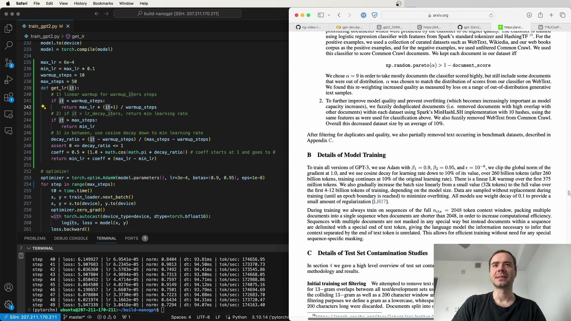
Elaborating on GPT-3 Training Details
For GPT-3, several specific training strategies are outlined:
- Adam Optimizer: The Adam optimizer is configured with
β1 = 0.9,β2 = 0.95, andϵ = 10^-8. - Gradient Clipping: The global norm of the gradients is clipped to 1.0.
- Cosine Decay: The learning rate is decayed to 10% of its original value over 260 billion tokens.
- LR Warmup: A linear learning rate warmup is applied over the first 375 million tokens.
- Batch Size Scaling: The batch size is gradually increased during the initial phase of training.
- Sequence Packing: To increase computational efficiency, multiple documents are packed into a single sequence when shorter than the full context window (
nctx = 2048tokens), with no special masking required.
These intricate details highlight the complexity and thoughtfulness that goes into training state-of-the-art language models like GPT-3. The process involves a fine balance between learning rate scheduling, data quality control, and optimization techniques. Through careful tuning and monitoring, these models can achieve remarkable performance on a wide range of tasks.
Understanding Batch Size Ramp-Up
In the realm of model optimization, one approach that has been discussed is the gradual increase in batch size—referred to as batch size ramp-up. This technique starts with a very small batch size and linearly increases it over time. However, we have chosen to skip this step for a couple of reasons:
- Batch size ramp-up complicates the arithmetic of the optimization process, as the number of tokens processed at each step changes.
- It is primarily a systems and speed optimization rather than an algorithmic one.
- In the early stages of training, the model is learning simple biases such as which tokens are used frequently and which are not, leading to highly correlated gradients across examples.
Consequently, we keep the batch size constant to maintain simplicity in our optimization calculations.
Sampling Data Without Replacement
Our training approach involves sampling data without replacement until an epoch boundary is reached. This means that once a sequence is drawn for training, it is not eligible to be drawn again until the next epoch. Our data loader iterates over chunks of data, exhausting a pool before moving on to the next set. Here’s how our custom DataLoaderLite class is structured:
class DataLoaderLite:
    def __init__(self, B, T):
        self.B = B  # Batch Size
        self.T = T  # Token Size

        # At initialization, load tokens from disk and store them in memory
        with open('input.txt', 'r') as f:
            text = f.read()
        enc = tokenizer.get_encoding('gpt2')
        tokens = enc.encode(text)
        tokens = torch.tensor(tokens)
        print(f'Total tokens loaded: {len(tokens)}')
This class ensures that once tokens are processed in a batch, they are not reused until the next epoch, thereby reducing the likelihood of overfitting.
Implementing Weight Decay
Weight decay is another tool in our optimization arsenal, providing a small amount of regularization to the model. We integrate this into our learning rate scheduler and optimizer configuration as follows:
# Learning rate and weight decay function
def get_lr(t, max_lr, min_lr, warmup_steps, max_steps):
    if t < warmup_steps:
        return max_lr * (t + 1) / warmup_steps
    decay_ratio = (t - warmup_steps) / (max_steps - warmup_steps)
    coeff = 0.5 * (1.0 + math.cos(math.pi * decay_ratio))
    return min_lr + coeff * (max_lr - min_lr)

# Configure optimizer with weight decay
def configure_optimizers(model, weight_decay=1e-1, learning_rate=6e-4, device):
    optimizer = torch.optim.AdamW(
        model.parameters(),
        lr=learning_rate,
        betas=(0.9, 0.95),
        eps=1e-8,
        weight_decay=weight_decay
    )
    return optimizer

# Example usage within the training loop
optimizer = configure_optimizers(model, 0.1, 6e-4, device)
The get_lr function is designed to adjust the learning rate using a cosine decay schedule, while the configure_optimizers function sets up our optimizer with the necessary parameters, including weight decay.
Training Loop Enhancements
Our enhanced training loop includes the configured learning rate scheduler and weight decay. We also keep track of the processing speed to monitor the model’s efficiency:
for step in range(max_steps):
    t0 = time.time()
    x, y = train_loader.next_batch()
    x, y = x.to(device), y.to(device)
    optimizer.zero_grad()
    with torch.autocast(device_type=device, dtype=torch.bfloat16):
        logits, loss = model(x, y)
    loss.backward()
    norm = torch.nn.utils.clip_grad_norm_(model.parameters(), 1.0)
    lr = get_lr(step, max_lr, min_lr, warmup_steps, max_steps)
    for param_group in optimizer.param_groups:
        param_group['lr'] = lr
    optimizer.step()
    torch.cuda.synchronize()  # Wait for GPU to finish work
    t1 = time.time()
    td = t1 - t0  # Time difference in seconds
    tokens_processed = train_loader.B * train_loader.T
    tokens_per_sec = tokens_processed / td
    # Output performance metrics
    print(f'step {step} loss: {loss.item():.6f} lr: {lr:.7f} | dt: {td*1000:.2f}ms | tok/sec: {tokens_per_sec:.2f}')
This training loop provides visibility into the model’s learning process, with clear metrics to analyze its performance in terms of loss, learning rate, processing time, and tokens processed per second.
GPT-3 Training Strategies
In the training of GPT-3, we adhere to the following practices:
- Adam Optimizer: Configured with β1 = 0.9, β2 = 0.95, and ε = 10^-8.
- Gradient Clipping: The global norm of the gradients is clipped to 1.0.
- Cosine Decay: The learning rate is decayed to 10% of its value over 260 billion tokens, continuing at this reduced rate thereafter.
- Linear Warmup: A warmup period is included over the first 375 million tokens.
- Data Sampling: We sample data without replacement during training to minimize overfitting.
- Weight Decay: A weight decay of 0.1 is used for regularization.
These strategies are encapsulated within our model’s configure_optimizers method:
class GPT(nn.Module):
    # ... model definition ...

    def configure_optimizers(self, weight_decay, learning_rate, device):
        # Start with all parameters that require gradients
        param_dict = {pn: p for pn, p in self.named_parameters() if p.requires_grad}
        # Group parameters for weight decay
        decay_params = [p for n, p in param_dict.items() if p.dim() > 2]
        nodecay_params = [p for n, p in param_dict.items() if p.dim() <= 2]
        optim_groups = [
            {'params': decay_params, 'weight_decay': weight_decay},
            {'params': nodecay_params, 'weight_decay': 0.0}
        ]
        optimizer = torch.optim.AdamW(
            optim_groups,
            lr=learning_rate,
            betas=(0.9, 0.95),
            eps=1e-8
        )
        return optimizer
The configure_optimizers method creates an optimizer with different parameter groups, some of which have weight decay applied. This nuanced approach allows us to tailor the regularization to the specific needs of different parts of the model.
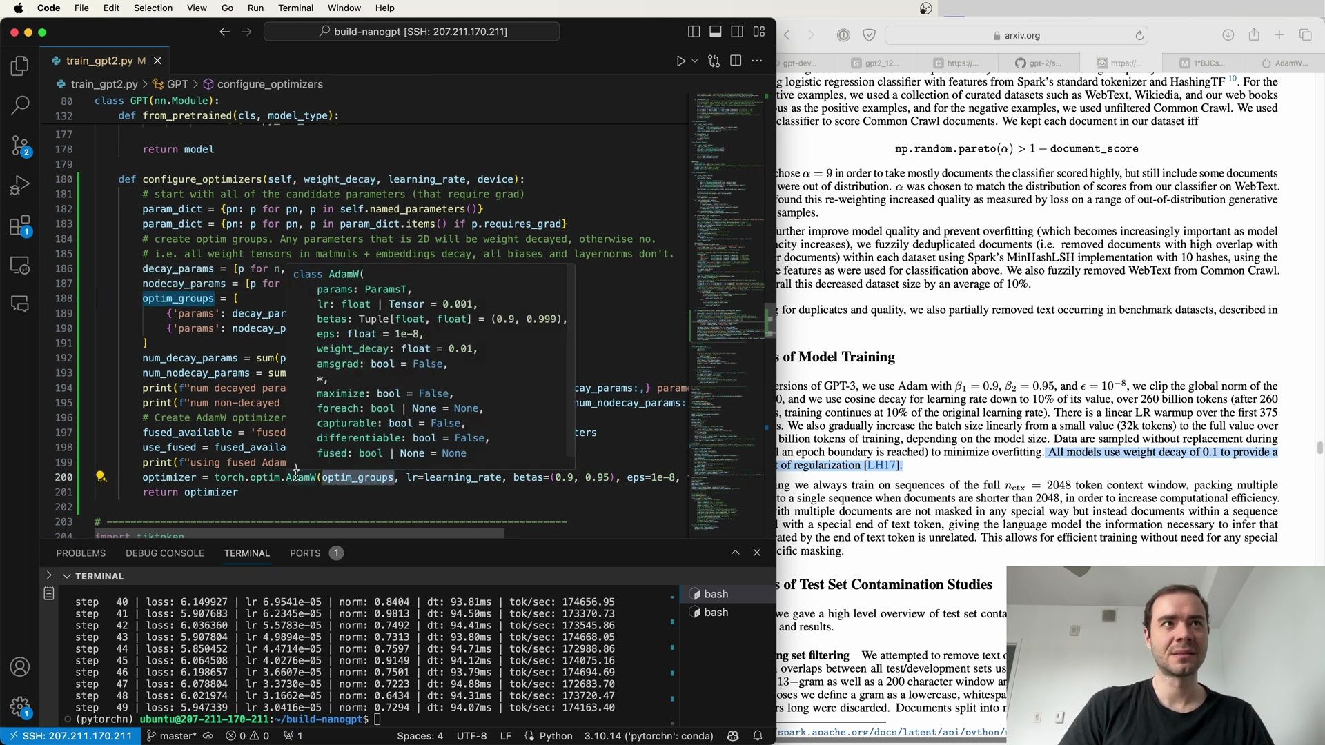
Fine-Tuning the Weight Decay Parameter
When configuring our optimizer, a key consideration is the weight_decay parameter. This parameter is essential for regularization, as it helps prevent individual weights from growing too large and encourages the distribution of importance across more neurons. In our implementation, this parameter is carefully fine-tuned and passed into a list of optimization groups, ultimately used by the AdamW optimizer.
The process involves segregating the model parameters into groups based on whether they should experience weight decay or not. Typically, biases and one-dimensional tensors, such as layer normalization scales, do not undergo weight decay. On the other hand, weights involved in matrix multiplications and embeddings are subject to decay. This distinction is made clear in the following code block, which details the configure_optimizers method of our GPT class:
class GPT(nn.Module):
    def configure_optimizers(self, weight_decay, learning_rate, device):
        # Start with all parameters that require gradients
        param_dict = {n: p for n, p in self.named_parameters() if p.requires_grad}
        # Split parameters into decay and no-decay groups
        decay_params = [p for n, p in param_dict.items() if p.dim() > 2]
        nodecay_params = [p for n, p in param_dict.items() if p.dim() <= 2]
        optim_groups = [
            {'params': decay_params, 'weight_decay': weight_decay},
            {'params': nodecay_params, 'weight_decay': 0.0}
        ]
        # Print the number of decay and no-decay parameters
        num_decay_params = sum(p.numel() for p in decay_params)
        num_nodecay_params = sum(p.numel() for p in nodecay_params)
        print(f'Using {num_decay_params} decay parameters and {num_nodecay_params} no-decay parameters')

        # Use the fused AdamW optimizer if available and running on CUDA
        fused_available = 'fused' in inspect.getsource(torch.optim.AdamW).parameters
        use_fused = fused_available and 'cuda' in device
        print(f'Using fused AdamW optimizer: {use_fused}')

        optimizer = torch.optim.AdamW(
            optim_groups,
            lr=learning_rate,
            betas=(0.9, 0.95),
            eps=1e-8
        )
        return optimizer
In the above method, we separate parameters into two lists: one for parameters that will undergo weight decay (decay_params) and one for parameters that will not (nodecay_params). The optimizer is then constructed with these two parameter groups, ensuring that only the appropriate parameters are regularized.
This nuanced approach allows the model to leverage the benefits of weight decay without negatively affecting parameters that should not be regularized, such as biases and normalization factors.
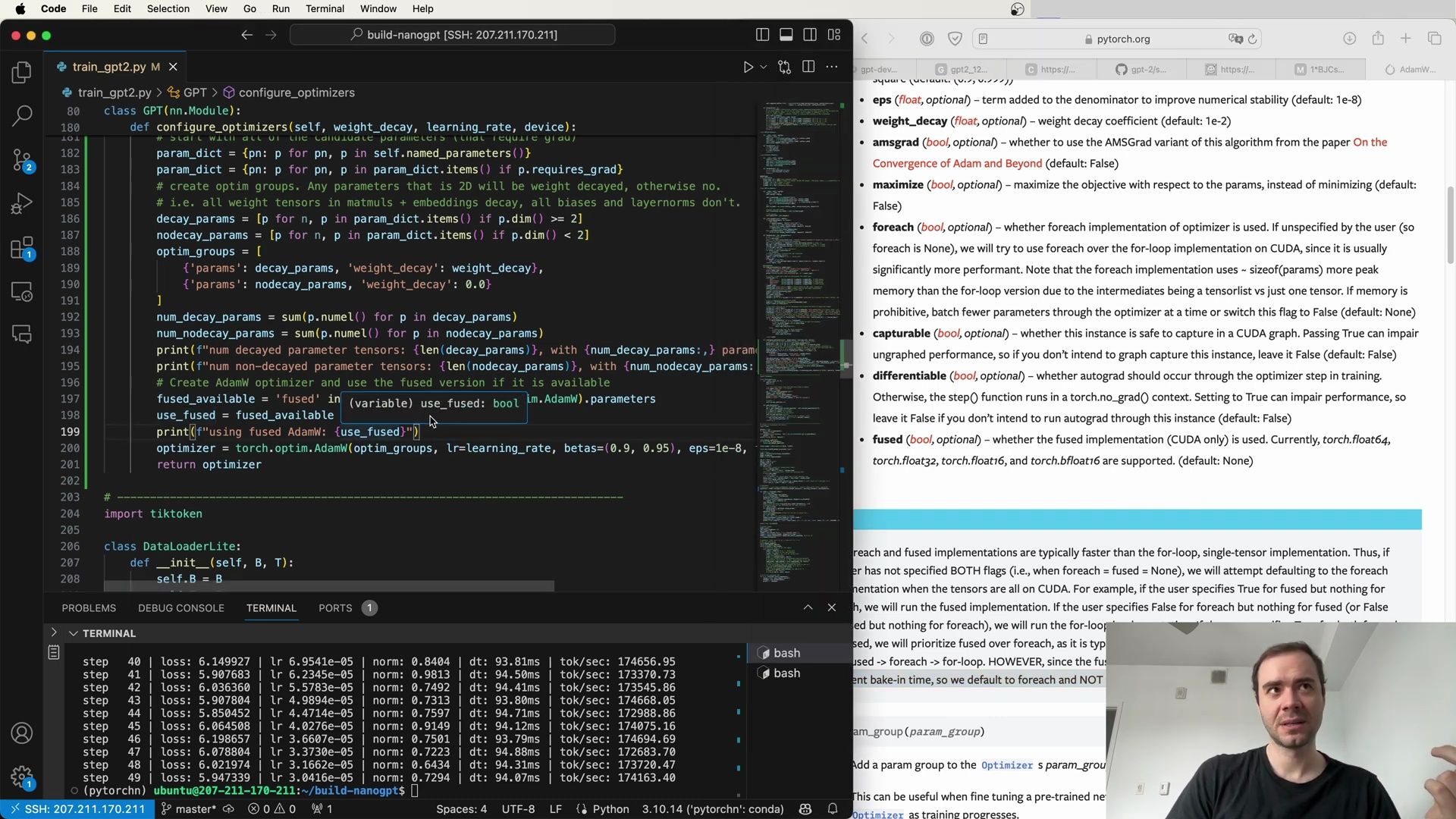
Leveraging Fused AdamW for Performance
An important optimization in our code is the use of the fused version of the AdamW optimizer when it’s available. This is a relatively new feature in PyTorch that can provide significant performance improvements, especially when running on CUDA-enabled devices. Fused AdamW essentially combines multiple operations into a single kernel call, which reduces the overhead of launching multiple kernels and can speed up the optimization process.
The following code snippet shows the detection of the fused AdamW optimizer and its conditional usage:
# ... within configure_optimizers method ...

# Check for the availability of the fused AdamW optimizer
fused_available = 'fused' in inspect.getsource(torch.optim.AdamW).parameters
use_fused = fused_available and 'cuda' in device
print(f'Using fused AdamW optimizer: {use_fused}')

# Create the AdamW optimizer, potentially using the fused version
optimizer = torch.optim.AdamW(
    optim_groups,
    lr=learning_rate,
    betas=(0.9, 0.95),
    eps=1e-8
)
return optimizer
By using the fused AdamW optimizer, we minimize the number of individual operations that need to be performed during each optimization step, leading to a more efficient training process.
Kernel Fusion Optimization
Kernel fusion is a technique that amalgamates several GPU kernel launches into a single launch. This can significantly reduce the computational overhead associated with the optimization step in training neural networks. When discussing the AdamW optimizer’s update step, we refer to kernel fusion as a method to streamline the update process across all parameter tensors. Instead of updating each tensor individually, which would result in multiple kernel launches, kernel fusion allows for a single kernel to update all parameters at once.
This optimization is particularly beneficial when using CUDA, as it maximizes the use of GPU resources and leads to faster execution times.
# ... within the configure_optimizers method ...

# Determine if the fused optimizer can be used
fused_available = 'fused' in inspect.getsource(torch.optim.AdamW).parameters
use_fused = fused_available and 'cuda' in device
print(f'Using fused AdamW optimizer: {use_fused}')

# The optimizer is instantiated with the option to use the fused variant if available
optimizer = torch.optim.AdamW(
    optim_groups,
    lr=learning_rate,
    betas=(0.9, 0.95),
    eps=1e-8
)
return optimizer
This method of optimization underscores the importance of staying up to date with advancements in machine learning libraries, as such updates can provide tangible benefits to model training efficiency.
Conclusion and Next Steps
As we continue to push the boundaries of neural network training, it’s crucial to fine-tune every aspect of the optimization process. From the careful selection of parameters that undergo weight decay to the adoption of fused kernel operations, each choice plays a role in enhancing the model’s performance. In the next section of our training journey, we will delve deeper into additional strategies and techniques that can further refine our model’s learning process. Stay tuned for more insights and code snippets that will help you master the art of neural network optimization.
Refining the configure_optimizers Method
Building upon our previous optimizer configuration, let’s delve into the specifics of the configure_optimizers method within our GPT class. This method plays a crucial role in distinguishing which parameters undergo weight decay and which do not. To ensure that our model performs at its best, we’ve got to be precise about how we apply weight decay.
Here’s an enhanced version of the configure_optimizers method:
class GPT(nn.Module):

    def configure_optimizers(self, weight_decay, learning_rate, device):
        # Start with all parameters that require gradients
        param_dict = {n: p for n, p in self.named_parameters() if p.requires_grad}
        # Split parameters into decay and no-decay groups
        # Weight tensors in matrix multiplications and embeddings will decay,
        # biases and layer norms will not
        decay_params = [p for n, p in param_dict.items() if p.dim() >= 2]
        nodecay_params = [p for n, p in param_dict.items() if p.dim() < 2]
        optim_groups = [
            {'params': decay_params, 'weight_decay': weight_decay},
            {'params': nodecay_params, 'weight_decay': 0.0}
        ]
        # Count the total number of decay and no-decay parameters
        num_decay_params = sum(p.numel() for p in decay_params)
        num_nodecay_params = sum(p.numel() for p in nodecay_params)
        # Print the parameter counts for debugging
        print(f"Decay params: {num_decay_params}, No-decay params: {num_nodecay_params}")

        # Use the fused AdamW optimizer if available and running on CUDA
        fused_available = 'fused' in inspect.getsource(torch.optim.AdamW).parameters
        use_fused = fused_available and 'cuda' in device
        print(f"Using fused AdamW optimizer: {use_fused}")

        optimizer = torch.optim.AdamW(
            optim_groups,
            lr=learning_rate,
            betas=(0.9, 0.95),
            eps=1e-8,
            use_fused=use_fused
        )
        return optimizer
As we can see from the script, the method begins by collecting all the trainable parameters. It then assigns these parameters to two distinct groups:
- Decay parameters: These are the weight tensors that are found in matrix multiplications and embeddings, which will undergo weight decay.
- No-decay parameters: These include biases and layer normalization scales, which will not undergo weight decay.
By segregating the parameters into these two categories, we can apply a different weight_decay value to each group, thereby ensuring that only the appropriate parameters are regularized.
One of the notable optimizations we’ve introduced is the conditional use of the fused version of the AdamW optimizer. We check for its availability and use it if we’re running on a CUDA-enabled device. The use of the fused optimizer can lead to substantial performance gains, as it combines multiple operations into fewer kernel calls.
Performance Improvements with Fused AdamW
The use of the fused AdamW optimizer can make a significant difference in training time. By reducing the number of kernel calls, we streamline the optimization step, allowing for a more efficient training loop. Even small improvements in run time per step can lead to substantial time savings over the entire training process.
Consider the following terminal output, which illustrates the performance improvement:
step 41 | loss: 5.097683 | lr: 6.7345e-05 | dt: 94.10ms | tok/sec: 173350.73
...
step 44 | loss: 5.084924 | lr: 6.7345e-05 | dt: 94.17ms | tok/sec: 174163.40
After implementing the fused version of AdamW, we observe a reduction in the time per step from 94 milliseconds to 90 milliseconds. This optimization results from the introduction of fused Adam and the decision to apply weight decay only to two-dimensional parameters like embeddings and matrices involved in linear transformations.
Emphasizing the Importance of Weight Decay Selection
To reiterate the significance of our weight decay strategy, it’s worth noting that most of the model’s parameters undergo decay. This is a deliberate choice, as it’s primarily the embeddings and weight matrices in matrix multiplications that require regularization to prevent overfitting. On the other hand, biases and layer normalization parameters, which are fewer in number, do not experience weight decay, as applying decay to these can negatively impact the model’s learning capacity.
Here’s a comparative look at the parameter counts:
- Number of decayed tensors: 50 (most of the parameters)
- Number of non-decayed tensors: 98 (biases and layers norms)
This careful balance ensures that our model remains robust and generalizes well to new data, without compromising on the ability to learn complex patterns.
In summary, the configure_optimizers function is a foundational piece of our training pipeline, setting the stage for an efficient and effective optimization process. By leveraging the latest features available in optimization algorithms and being selective about which parameters undergo weight decay, we’re optimizing not just the model’s performance but also our training efficiency.
Learning Rate Scheduling and Optimization
Optimizing the learning rate schedule is a key aspect of training neural networks effectively. The get_lr function provided in the script is a crucial component of such a schedule. It defines three phases of learning rate adjustments: linear warmup, cosine decay, and a constant minimum learning rate.
Here’s the get_lr function as described:
def get_lr(it):
    # 1) linear warmup for warmup_steps steps
    if it < warmup_steps:
        return max_lr * (it+1) / warmup_steps
    # 2) if it > max_steps, return minimum learning rate
    if it > max_steps:
        return min_lr
    # 3) in between, use cosine decay down to min learning rate
    decay_ratio = (it - warmup_steps) / (max_steps - warmup_steps)
    assert decay_ratio >= 0
    coeff = 0.5 * (1.0 + math.cos(math.pi * decay_ratio))
    return max_lr * coeff
In the training loop, we see the model’s optimizer configured with a specific weight decay and learning rate. An important note is made regarding the efficiency of different implementations of optimizers. Specifically, the text points out that the foreach and fused implementations typically offer greater speed than the traditional for-loop, single-tensor implementations. It also emphasizes the use of the foreach implementation as the default when the tensors reside on CUDA devices.
The following code snippet shows the training loop where the optimizer is used, and the learning rate is updated at each step:
optimizer = model.configure_optimizers(weight_decay=0.1, learning_rate=6e-4, device=device)

for step in range(max_steps):
    t0 = time.time()
    x, y = train_loader.next_batch()
    x, y = x.to(device), y.to(device)
    optimizer.zero_grad()
    with torch.autocast(device_type=device, dtype=torch.bfloat16):
        logits, loss = model(x, y)
    loss.backward()
    norm = torch.nn.utils.clip_grad_norm_(model.parameters(), 1.0)
    # determine and set the learning rate for this iteration
    lr = get_lr(step)
    for param_group in optimizer.param_groups:
        param_group['lr'] = lr
    optimizer.step()
    t1 = time.time()
    print(f'step {step+1}/{max_steps}, dt: {t1-t0:.2f}s, tok/sec: {int(y.numel()/(t1-t0))}')
From the terminal output, we can see the learning rate is dynamically adjusted, leading to changes in the loss over time:
step 35 loss=0.6972, lr=0.000751, dt: 0.93s, tok/sec: 181974.72
...
step 47 loss=0.4870, lr=0.000739, dt: 0.89s, tok/sec: 181277.02
Advanced Optimizer Configurations
The script further discusses the importance of fine-tuning the optimizer settings when dealing with pre-trained models. The add_param_group method is highlighted as a tool for updating the optimizer with new parameter groups, which is often necessary when different parts of the model are fine-tuned with varying learning rates.
In the context of model training, the script outlines the approach used for training GPT-3 models:
- Adam Optimizer Settings: The models are trained using the Adam optimizer with β1 = 0.9, β2 = 0.95, and ϵ = 10^-8.
- Gradient Clipping: The global norm of the gradients is clipped at 1.0 to prevent exploding gradients.
- Learning Rate Scheduling: A cosine decay is used for the learning rate, reducing it to 10% of its value over a vast number of tokens.
- Batch Size Scaling: The batch size is gradually increased linearly from a smaller value to the full value over billions of tokens, depending on the model size.
- Data Sampling: To minimize overfitting, data are sampled without replacement during training.
These strategies are complemented by other details like document packing for efficiency and the use of a special end-of-text token to denote document boundaries within sequences.
Evaluation of GPT-3 on NLP Tasks
The evaluation of GPT-3 on various natural language processing tasks reveals insights into its capabilities:
- Reading Comprehension: GPT-3’s performance varies significantly across different datasets, suggesting its adaptability to different answer formats.
- SuperGLUE Benchmark: GPT-3 is also assessed on the SuperGLUE benchmark, a standardized collection of datasets, to compare its performance against models like BERT and RoBERTa.
In summary, the script and the extracted content from the images offer a deep dive into the detailed configurations and considerations necessary for effectively training and evaluating large-scale language models like GPT-3. Optimizations in learning rate scheduling, optimizer configurations, and evaluation methodologies contribute to the model’s overall performance and its ability to generalize across a wide range of tasks.
Model Size and Learning Rate Adaptations
As we delve deeper into the nuances of transformer-based models, we recognize that various hyperparameters require fine-tuning to optimize performance. The relationship between the size of the model and the learning rate is particularly pivotal. Generally, larger networks are trained with slightly lower learning rates, and the batch size tends to increase alongside the model’s size.
The trade-off between computational resources and the optimal hyperparameters is a constant challenge in the field of deep learning. For instance, a batch size of 0.5 million may be ideal for some large networks, but it’s impractical for individuals or organizations with limited GPU capabilities. However, the goal remains to emulate the conditions that these hyperparameters provide.
Gradient Accumulation: A Solution for Limited Resources
One effective strategy to overcome resource limitations is gradient accumulation. This technique allows us to simulate large batch sizes on smaller GPUs by running multiple forward and backward passes before performing a parameter update. Here’s how it works:
# total desired batch size (0.5 million tokens)
total_batch_size = 524288 # roughly 2**19
# micro batch size (number of tokens processed in a single forward/backward pass)
micro_batch_size = 16
# sequence length
sequence_length = 1024
# calculate gradient accumulation steps
grad_accum_steps = total_batch_size // (micro_batch_size * sequence_length)
By setting a micro_batch_size and calculating the number of gradient accumulation steps (grad_accum_steps), we can process a more extensive set of tokens across several iterations before updating the model parameters. This allows for the simulation of larger batch sizes without exceeding GPU memory limits.
Implementing Gradient Accumulation in the Training Loop
Let’s now integrate the gradient accumulation strategy into our training loop. The following code snippet demonstrates how to adjust the training loop to accommodate this method:
# Configure the device for training
device = 'cuda' if torch.cuda.is_available() else 'cpu'
print(f'Using device: {device}')

# Seed setting for reproducibility
torch.manual_seed(1337)
if torch.cuda.is_available():
    torch.cuda.manual_seed(1337)

# DataLoader configuration
train_loader = DataLoaderLite(B=micro_batch_size, T=sequence_length)

# Model configuration
model = GPT(GPTConfig(vocab_size=50304))
model.to(device)
model = torch.compile(model)

# Learning rate configuration
max_lr = 6e-4
min_lr = max_lr * 0.1
warmup_steps = 10
max_steps = 50

# Begin the training loop
for step in range(max_steps):
    optimizer.zero_grad()
    for _ in range(grad_accum_steps):
        x, y = train_loader.next_batch()
        x, y = x.to(device), y.to(device)
        with torch.autocast(device_type=device, dtype=torch.bfloat16):
            logits, loss = model(x, y)
        loss.backward()
    # Update model parameters after accumulating gradients
    optimizer.step()
In the modified training loop, each micro_batch is processed through the forward and backward pass, gradients are accumulated, and after grad_accum_steps iterations, the parameters are updated.
Model Architectures Across Different Scales
When examining the architecture of models trained for this research, we note a range of model sizes, from 125 million parameters all the way up to the 175 billion parameters of GPT-3. Each of these models has been trained for a total of 300 billion tokens, showcasing the scalability of the transformer architecture.
The various models share a common structure, taken from GPT-2, which includes modified initialization, pre-normalization, and attention bias. However, some adaptations have been made, such as alternating dense and locally banded sparse attention patterns, which contribute to the models’ efficiency and performance.
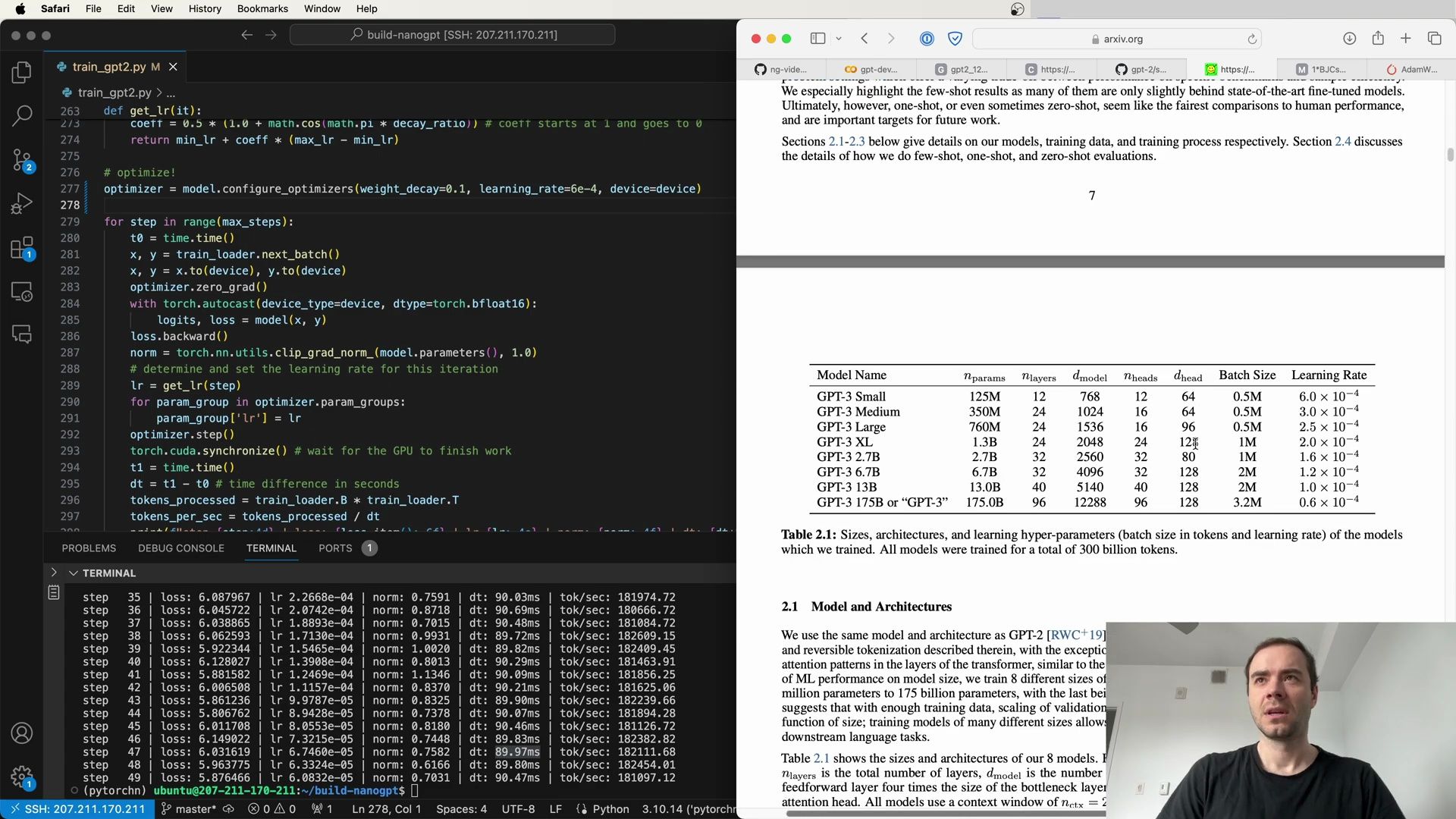
Hyperparameters Across Model Sizes
The following table provides a summary of the learning hyperparameters for different model sizes:
- Small (125M parameters): Batch Size: 0.5M, Learning Rate: 6.0 x 10^-4
- Medium (350M parameters): Batch Size: 0.5M, Learning Rate: 3.0 x 10^-4
- Large (760M parameters): Batch Size: 0.5M, Learning Rate: 2.5 x 10^-4
- XL (1.3B parameters): Batch Size: 1M, Learning Rate: 2.0 x 10^-4
- 2.7B parameters: Batch Size: 1M, Learning Rate: 1.6 x 10^-4
- 6.7B parameters: Batch Size: 2M, Learning Rate: 1.2 x 10^-4
- 13B parameters: Batch Size: 2M, Learning Rate: 1.0 x 10^-4
- GPT-3 (175B parameters): Batch Size: 3.2M, Learning Rate: 0.6 x 10^-4
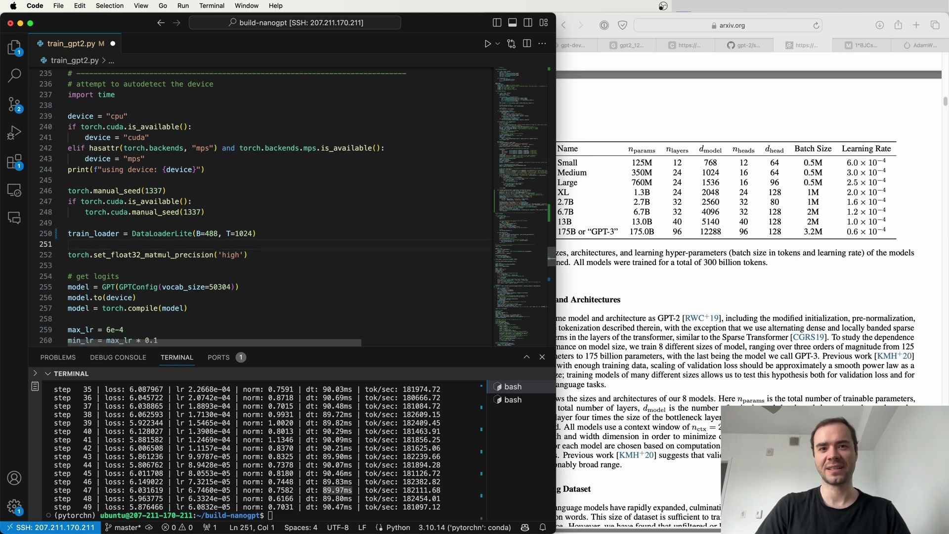
Each model has been chosen based on computational efficiency and performance, with all models using a context window (n_ctx) of 2048 and a bottleneck dimension (neck_size) of 128. The sizes and architectures of these models are chosen within a reasonably broad range to facilitate a variety of computational capabilities and research objectives.
Conclusion
In summary, the meticulous optimization of learning rates, batch sizes, and model architectures is paramount for the successful training of large-scale language models. Techniques such as gradient accumulation provide a pathway for those with limited computational resources to participate in this research. The findings from these diverse models offer valuable insights into the scalability and performance of transformer networks, serving as a foundation for future advancements in the field.
Customizing the Learning Rate Schedule
In the context of training large models, the learning rate schedule plays a crucial role in achieving convergence and fine-tuning the model’s performance. A popular approach is to use a cosine decay schedule for the learning rate, which starts high and gradually decreases following a cosine curve. This method is often preferred because it allows for large initial learning rates for faster convergence, while slowly fine-tuning the weights as training progresses.
Let’s examine the implementation of a cosine decay learning rate schedule:
import math

def get_lr(t, warmup_steps, max_steps, min_lr, max_lr):
    # 3) Between the warmup and max_steps, use cosine decay down to min learning rate
    decay_ratio = (t - warmup_steps) / (max_steps - warmup_steps)
    assert 0 <= decay_ratio <= 1
    coeff = 0.5 * (1.0 + math.cos(math.pi * decay_ratio))  # coeff starts at 1 and decays to 0
    return min_lr + (max_lr - min_lr) * coeff
Here, t represents the current timestep, warmup_steps is the number of steps during which the learning rate linearly increases to max_lr, and max_steps is the total number of training steps. The min_lr and max_lr are the minimum and maximum learning rates, respectively.
Optimizer Configuration and Learning Rate Application
With the learning rate schedule defined, we can now configure the optimizer and apply the learning rate dynamically at each step of training:
optimizer = model.configure_optimizers(weight_decay=0.1, learning_rate=6e-4)

# Training loop
for step in range(max_steps):
    # Measure the time for performance metrics
    t0 = time.time()

    # Reset gradients to zero before starting accumulation
    optimizer.zero_grad()

    # Inner loop for gradient accumulation
    for micro_step in range(grad_accum_steps):
        x, y = train_loader.next_batch()
        x, y = x.to(device), y.to(device)
        with torch.autocast(device_type=device, dtype=torch.bfloat16):
            logits, loss = model(x, y)
        loss.backward()

    # Clip gradients to a specified norm
    norms = torch.nn.utils.clip_grad_norm_(model.parameters(), 1.0)

    # Determine and set the learning rate for this iteration
    lr = get_lr(step, warmup_steps, max_steps, min_lr, max_lr)
    for param_group in optimizer.param_groups:
        param_group['lr'] = lr

    # Perform an optimization step
    optimizer.step()

    # Wait for the GPU to finish work before proceeding to the next step
    torch.cuda.synchronize()

    # Calculate elapsed time and throughput
    t1 = time.time()
    dt = t1 - t0
    tokens_processed = train_loader.B * train_loader.T
    tokens_per_sec = tokens_processed / dt

    # Log training progress
    print(f'step {step:4d}: loss: {loss.item():.4f} | lr {lr:.4e} | norm {norms:.4f} | dt {dt:.4f}s | tokens/sec: {tokens_per_sec:.0f}')
In this code snippet, optimizer is configured with weight decay and an initial learning rate. Inside the training loop, we perform gradient accumulation, clip gradients to prevent exploding gradients, and then apply the scheduled learning rate for the current timestep before updating the model’s parameters.
Understanding Gradient Accumulation Mechanism
Gradient accumulation is a useful technique when dealing with the constraint of limited GPU memory. It allows for simulating larger batch sizes by accumulating gradients over several mini-batches before updating the model parameters. To clarify the concept, let’s consider a simple neural network example using PyTorch:
import torch

# Simple MLP model
net = torch.nn.Sequential(
    torch.nn.Linear(16, 32),
    torch.nn.GELU(),
    torch.nn.Linear(32, 1)
)
torch.random.manual_seed(42)
x = torch.randn(4, 16)  # Random examples
y = torch.randn(4, 1)   # Target values

# Zero gradients before backward pass
net.zero_grad()

# Forward pass
yhat = net(x)
# Compute loss using Mean Squared Error (MSE)
loss = torch.nn.functional.mse_loss(yhat, y)
# Backward pass (gradient calculation)
loss.backward()

# Print out gradient of the first layer
print(net[0].weight.grad.view(-1)[:10])
The above code constructs a simple Multi-Layer Perceptron (MLP) and performs a forward and backward pass with a batch of four examples. The loss used here is the mean squared error (MSE), and we print out the gradient of the weights in the first layer.
The Impact of Reduction on Loss Calculation
When calculating the loss, the reduction method used can significantly impact the gradients. By default, the mse_loss function in PyTorch uses a mean reduction, averaging the loss over all examples in the batch:
# Loss objective with mean reduction (default)
# L = 1/4 * ((y[0] - yhat[0])**2 + (y[1] - yhat[1])**2 + (y[2] - yhat[2])**2 + (y[3] - yhat[3])**2)
However, when using gradient accumulation, the reduction method needs to change. Instead of averaging the loss across the batch, we sum the loss for each example to ensure proper scaling during accumulation:
# Accumulated loss objective (sum reduction)
# L = (y[0] - yhat[0])**2 + (y[1] - yhat[1])**2 + (y[2] - yhat[2])**2 + (y[3] - yhat[3])**2
In the context of gradient accumulation, it’s crucial to modify the loss calculation accordingly. Hence, the PyTorch code for the loss calculation with sum reduction would look like this:
# Compute loss using Mean Squared Error (MSE) with sum reduction
loss = torch.nn.functional.mse_loss(yhat, y, reduction='sum')
loss.backward()  # Backward pass for gradient accumulation
This adjustment ensures that the accumulated gradients reflect the sum of the losses over the mini-batches, which is equivalent to using a larger batch size.
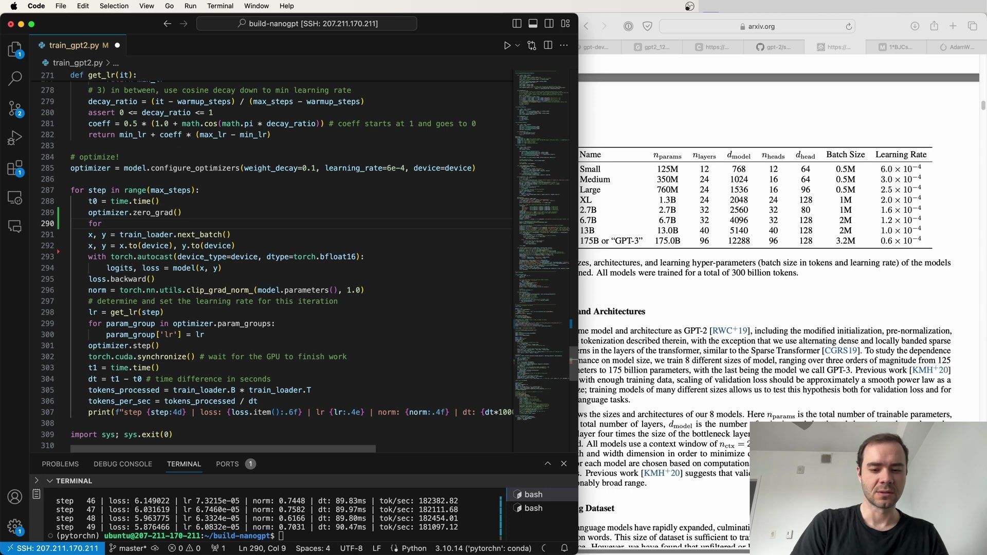
In conclusion, understanding and implementing an effective learning rate schedule and gradient accumulation strategy are essential for training large-scale models efficiently and effectively. With these techniques, researchers and practitioners can tackle computational constraints and optimize their models’ performance.
Fine-tuning the Learning Rate Function
Expanding on the learning rate schedule, we’ve previously discussed the get_lr function, which is where the bulk of our learning rate schedule logic is contained. This function not only takes care of the warm-up phase but also implements cosine decay for the learning rate. Let’s revisit and refine our get_lr function as follows:
def get_lr(t, warmup_steps, max_steps, min_lr, max_lr):
    # 1) lr warm-up from min to max
    # 2) stay at max
    # 3) ln between, use cosine decay down to min learning rate
    assert t >= 0 and max_steps >= warmup_steps
    if t < warmup_steps:
        lr = min_lr + (max_lr - min_lr) * (t / warmup_steps)
    elif t < max_steps:
        decay_ratio = (t - warmup_steps) / (max_steps - warmup_steps)
        assert 0 <= decay_ratio <= 1
        coeff = 0.5 * (1.0 + math.cos(math.pi * decay_ratio)) # coeff starts at 1 and goes down to 0
        lr = min_lr + coeff * (max_lr - min_lr)
    else:
        lr = min_lr
    return lr
This refined function now handles three distinct phases of the learning rate: the warm-up phase, the high learning rate phase, and the cosine decay phase. It’s important to note the assertions in the function that validate our assumptions about the time step t and max_steps.
Implementing and Applying the Learning Rate Schedule
Now, we will put our learning rate function to work within the training loop. We configure our optimizer with a weight decay, a starting learning rate, and specify the type of decay we’re going to use, which in this case is ‘cosine’:
# optimizer configuration with cosine decay
optimizer = model.configure_optimizers(weight_decay=0.1, learning_rate=6e-4, decay_type='cosine')

# Training loop
for step in range(max_steps):
    t0 = time.time()
    optimizer.zero_grad()

    # Inner loop for gradient accumulation
    for micro_step in range(grad_accum_steps):
        X, y = train_loader.next_batch()
        X, y = X.to(device), y.to(device)
        with torch.autocast(device_type=device, dtype=torch.float16):
            logits, loss = model(X, y)
        loss.backward()

    # Clip gradients
    torch.nn.utils.clip_grad_norm_(model.parameters(), 1.0)

    # Set and apply the learning rate for the current step
    lr = get_lr(step, warmup_steps, max_steps, min_lr, max_lr)
    for param_group in optimizer.param_groups:
        param_group['lr'] = lr

    optimizer.step()
    torch.cuda.synchronize()  # Ensure all operations are finished
    t1 = time.time()
    dt = t1 - t0

    tokens_processed = train_loader.B * train_loader.T
    tokens_per_sec = tokens_processed / dt

    # Logging training metrics
    print(f'step {step:4d}: loss: {loss.item():.4f} | lr {lr:.4e} | norm: {torch.nn.utils.clip_grad_norm_(model.parameters(), 1.0):.4f}')
In the above code, we have a training loop that zeroes out the gradients, performs a backward pass with gradient accumulation, clips gradients to avoid exploding gradients, sets the learning rate for the current iteration, and steps the optimizer to update the model’s weights.
Gradient Accumulation and Loss Normalization
When employing gradient accumulation, it is imperative to adjust the loss calculation. Unlike the default mean reduction, we need to use a sum reduction to accumulate gradients correctly. This means we should not average the loss over the accumulation steps but rather sum it up. This adjustment is essential to emulate the effect of a larger batch size. Here’s how it looks in code:
# Forward pass and calculate loss with sum reduction
yhat = net(x)
loss = torch.nn.functional.mse_loss(yhat, y, reduction='sum')
loss.backward()  # Backward pass for gradient accumulation

# ... rest of the training loop ...
In the above snippet, setting reduction='sum' in the mse_loss function ensures that the loss is not averaged across the batch, which is crucial for the gradient accumulation process.
Real-time Training Metrics Output
To monitor the training process and ensure everything is progressing smoothly, we output key metrics at each step of the training loop. These metrics include the current loss, the applied learning rate, the gradient norm, and the processing speed in terms of tokens per second:
print(f'step {step:4d}: loss: {loss.item():.4f} | lr {lr:.4e} | norm: {torch.nn.utils.clip_grad_norm_(model.parameters(), 1.0):.4f} | dt: {dt:.2f}s | tok/sec: {tokens_per_sec:.0f}')
This output helps us to keep an eye on the training process and diagnose any potential issues early on.
The mechanisms of learning rate scheduling and gradient accumulation are complex yet vital elements in the training of large models. By understanding and implementing these techniques, we can exert fine control over the training process, helping our models to learn effectively within the constraints of our computational resources.
Adjusting Loss Calculation for Gradient Accumulation
In our training regimen, when applying gradient accumulation, it’s crucial to adjust the loss calculation accordingly. Rather than using the mean reduction, we sum the losses over the accumulation steps. This modification is vital to accurately emulate the effect of a larger batch size, as gradient accumulation is effectively a sum of gradients over multiple forward passes. The code below demonstrates how to adjust the loss calculation for gradient accumulation:
# Forward pass and calculate loss with sum reduction for gradient accumulation
loss = 0
for micro_step in range(grad_accum_steps):
    X, y = train_loader.next_batch()
    X, y = X.to(device), y.to(device)
    with torch.autocast(device_type=device, dtype=torch.float16):
        logits, yhat = model(X)
        loss += torch.nn.functional.mse_loss(yhat, y, reduction='sum')
loss.backward()  # Backward pass for gradient accumulation
With the above adjustment, each individual loss is added together to form the accumulated loss. However, this means that the loss will scale with the number of accumulation steps, leading to larger gradient values. To counteract this, we introduce normalization by dividing the accumulated loss by the number of accumulation steps:
# Normalize the accumulated loss
loss /= grad_accum_steps
By scaling the loss in this manner, each individual loss contribution is effectively weighted equally regardless of the number of accumulation steps, ensuring that the gradients remain consistent.
Correcting Gradient Values with Loss Scaling
It’s important to scale the loss correctly to ensure that the gradients are comparable to those obtained from a larger batch size without accumulation. Here’s how we integrate this into our training loop:
# Training loop with normalization of accumulated loss
for step in range(max_steps):
    optimizer.zero_grad()
    loss = 0
    for micro_step in range(grad_accum_steps):
        X, y = train_loader.next_batch()
        X, y = X.to(device), y.to(device)
        with torch.autocast(device_type=device, dtype=torch.float16):
            logits, yhat = model(X)
            loss += torch.nn.functional.mse_loss(yhat, y, reduction='sum')
    loss /= grad_accum_steps  # Normalize the loss
    loss.backward()
    nn.utils.clip_grad_norm_(model.parameters(), 1.0)

    # Determine and set the learning rate for this iteration
    lr = get_lr(step)
    for param_group in optimizer.param_groups:
        param_group['lr'] = lr
    optimizer.step()
    print(f'step {step:4d}: loss: {loss.item():.4f} | lr {lr:.4e} | norm: {nn.utils.clip_grad_norm_(model.parameters(), 1.0):.4f}')
In the snippet above, we’ve normalized the loss before the backward pass. This ensures that the gradients are scaled down appropriately, and the update step will be consistent with the expected gradient values as if we had used a larger batch size.
Detailed Example of Loss Scaling with Gradient Accumulation
To illustrate the effect of loss scaling, let’s consider a more detailed example with explicit calculation of each loss component:
# Calculate each loss component explicitly with scaling
losses = []
for i in range(grad_accum_steps):
    y_i = y[i]
    yhat_i = yhat[i]
    L_i = 1/4 * (y_i - yhat_i)**2  # Scale each loss component
    losses.append(L_i)

# Sum the scaled loss components
loss = sum(losses)

# Now proceed with the backward pass and optimizer step as usual
loss.backward()
nn.utils.clip_grad_norm_(model.parameters(), 1.0)
optimizer.step()
In the code above, each loss component L_i is scaled by a factor of 1/4, which corresponds to the inverse of the number of gradient accumulation steps (grad_accum_steps = 4). This scaling ensures that the accumulated gradient is equivalent to the gradient that would result from a single pass with a batch size equal to the number of accumulation steps.
By implementing these adjustments in our training loop, we achieve consistent and correct gradient values, enabling our model to learn effectively without the computational burden of large batch sizes. This technique is especially useful when working with large models or limited hardware resources.
Implementing a GPT Model Class
When constructing a model class for GPT, we extend from nn.Module. The initialization of the class requires the number of classes cls and the model_type. The structure of the model class might look something like this:
class GPT(nn.Module):
    def __init__(self, cls, model_type):
        # ... initialization code ...
The forward method of the model class is where the computation takes place. We process the input indices idx and, if provided, calculate the loss against the targets. The forward method could be defined as follows:
class GPT(nn.Module):
    def forward(self, idx, targets=None):
        # ... [code truncated] ...
        x = self.tran(x)
        logits = self.lm_head(x)
        loss = None
        if targets is not None:
            loss = F.cross_entropy(logits.view(-1, logits.size(-1)), targets.view(-1))
            return logits, loss
For convenience, we can also include a class method to easily create a model with pretrained weights:
@classmethod
def from_pretrained(cls, model_type):
    # ... code to load pretrained weights ...
Loss Calculation with Cross Entropy
In a GPT model, loss calculation is often performed using cross-entropy loss. However, it is important to note that the default reduction in the cross-entropy function is typically mean. This means that the loss would be averaged over all elements:
loss = F.cross_entropy(logits.view(-1, logits.size(-1)), targets.view(-1), reduction='mean')
Learning Rate Scheduling
The learning rate scheduling can significantly affect the training process. Suppose we define a function get_lr which takes the current timestep t and computes the learning rate based on linear warmup and cosine decay:
def get_lr(t):
    # Linear warmup
    if t < warmup_steps:
        return max_lr * (t+1) / warmup_steps
    # Constant learning rate after warmup until max_steps
    if t > max_steps:
        return min_lr
    # Cosine decay down to min learning rate
    decay_ratio = (t - warmup_steps) / (max_steps - warmup_steps)
    assert 0 <= decay_ratio <= 1
    coeff = 0.5 * (1.0 + math.cos(math.pi * decay_ratio))
    return min_lr + coeff * (max_lr - min_lr)
This learning rate is then applied within the training loop. Each optimizer step is preceded by the computation and setting of the current learning rate:
optimizer = model.configure_optimizers(weight_decay=0.1, learning_rate=6e-4, decay=0.05)

for step in range(max_steps):
    optimizer.zero_grad()
    # ... training steps ...
    lr = get_lr(step)
    for param_group in optimizer.param_groups:
        param_group['lr'] = lr
    optimizer.step()
Scaling Loss for Gradient Accumulation
As discussed earlier, it’s crucial to scale the loss when using gradient accumulation to ensure that gradients are appropriately normalized. This can be done by dividing the loss by the number of gradient accumulation steps:
for micro_step in range(grad_accum_steps):
    # ... forward pass ...
    loss = loss / grad_accum_steps
loss.backward()
Detailed Loss Calculation with Gradient Accumulation
Let’s consider a more detailed example where each loss component is explicitly calculated and scaled. Assuming that we’re using a batch size B=1 and gradient accumulation steps of 4, we compute the loss as follows:
import torch

# Assuming grad_accum_steps of 4, and B=1
# Accumulation in gradient corresponds to a SUM in loss
# We compute each loss component and scale it
L0 = 1/4 * (y[0] - yhat[0])**2
L1 = 1/4 * (y[1] - yhat[1])**2
L2 = 1/4 * (y[2] - yhat[2])**2
L3 = 1/4 * (y[3] - yhat[3])**2
# The total loss is the sum of the individual scaled losses
L = L0 + L1 + L2 + L3
This loss computation ensures that the gradient resulting from loss.backward() will be equivalent to the gradient obtained from a single forward pass with a batch size equal to the number of accumulation steps.
Training Loop with Scaled Loss and Learning Rate Scheduling
In the training loop, we integrate loss scaling and learning rate scheduling to optimize the model:
for step in range(max_steps):
    # Track time for performance metrics
    t0 = time.time()
    optimizer.zero_grad()
    loss_accum = 0.0

    for micro_step in range(grad_accum_steps):
        # Perform forward and backward passes
        x, y = train_loader.next_batch()
        x, y = x.to(device), y.to(device)
        with torch.autocast(device_type=device, dtype=torch.float16):
            logits, loss = model(x, y)
            loss = loss / grad_accum_steps
        loss_accum += loss.detach()
        loss.backward()

    # Clip gradients and perform an optimizer step
    norm = torch.nn.utils.clip_grad_norm_(model.parameters(), 1.0)
    lr = get_lr(step)
    for param_group in optimizer.param_groups:
        param_group['lr'] = lr
    optimizer.step()
    torch.cuda.synchronize() # wait for the GPU to finish work
    t1 = time.time()
By carefully scaling the loss and adjusting the learning rate, we ensure that the training loop is robust and conducive to learning.
Real-time Performance Metrics
During training, it’s useful to have real-time metrics to monitor the progress and performance. These can include the learning rate, loss, and speed of processing tokens:
    # Calculate tokens processed per second
    tokens_processed = train_loader.B * train_loader.T
    tokens_per_sec = tokens_processed / (t1 - t0)
    print(f'step {step} lr {lr:.5f} loss {loss:.5f} dt {t1 - t0:.3f} tok/sec: {tokens_per_sec:.2f}')
By providing these insights, we can make informed decisions about adjusting the training process and diagnosing potential issues.
Accumulating Loss for Gradient Descent
In order to optimize our GPT model effectively, we need to carefully manage how we accumulate loss during gradient descent. Since we’re working with potentially very large datasets and models, it might be impractical to compute the loss over the entire dataset at once. Instead, we use a technique called gradient accumulation to approximate the same effect.
When accumulating gradients, we must adjust how we calculate and apply the loss. In our training loop, we not only need to accumulate the loss over several forward and backward passes but also need to ensure that the gradients are scaled appropriately. This is because each call to loss.backward() will add gradients to the already stored values, effectively summing them up, when what we actually want is their mean.
Here’s how we might implement this in our training loop:
# train_gpt2.py
# Initialize loss accumulation variable
loss_accum = 0.0

# Loop over the range of steps we want to train for
for step in range(max_steps):
    optimizer.zero_grad()  # Clear any previously calculated gradients

    # Perform forward and backward passes multiple times
    for micro_step in range(grad_accum_steps):
        x, y = train_loader.next_batch()  # Get the next batch of data
        x, y = x.to(device), y.to(device)  # Move the data to the proper device
        with torch.autocast(device_type=device, dtype=torch.bfloat16):
            logits, loss = model(x, y)
            # Scale the loss to account for the addition of gradients
            loss = loss / grad_accum_steps
            loss_accum += loss.detach()  # Accumulate the scaled loss
        loss.backward()  # Compute gradients

    # Clip the gradients to avoid exploding gradient problem
    norm = torch.nn.utils.clip_grad_norm_(model.parameters(), 1.0)

    # Adjust the learning rate based on the scheduling function
    lr = get_lr(step)
    for param_group in optimizer.param_groups:
        param_group['lr'] = lr
    optimizer.step()  # Update model parameters
As we’re accumulating the loss, we must also consider the total number of tokens processed, especially when working with variable batch sizes due to gradient accumulation. This allows us to calculate metrics like tokens per second, giving us insight into the training speed:
# Calculate the time difference between the start and end of the training step
dt = t1 - t0

# Update the total tokens processed, taking the gradient accumulation into account
tokens_processed += train_loader.batch_size * grad_accum_steps

# Calculate the number of tokens processed per second
tokens_per_sec = tokens_processed / dt

# Output the training step information
print(f'step {step:4d}: loss={loss.item():.6f} | lr {lr:.4e} | norm={norm:.4e} | tokens_per_sec={tokens_per_sec:.2f}')
Understanding Loss Calculation with Gradient Accumulation
The concept of gradient accumulation can be a bit abstract, so let’s clarify how the loss is calculated in this context. Typically, we’d calculate the loss for a batch and then perform backpropagation. However, with gradient accumulation, we’re summing the gradients over multiple smaller batches (micro-steps) before updating the parameters.
Here’s a more detailed breakdown of the loss calculation with gradient accumulation steps of 4, and a batch size B=1:
# For each micro-batch, we compute the loss component and scale it
L0 = 1/4 * (y[0] - yhat[0])**2
L1 = 1/4 * (y[1] - yhat[1])**2
L2 = 1/4 * (y[2] - yhat[2])**2
L3 = 1/4 * (y[3] - yhat[3])**2

# The total loss is the sum of the individual scaled losses
L = L0 + L1 + L2 + L3
By scaling each individual loss component by the number of gradient accumulation steps (in this case, 4), we ensure that the effect on the gradients is equivalent to computing the loss on a batch size equal to the number of accumulation steps.
Real-time Training Metrics
As we run our training loop, it’s important to keep an eye on performance metrics in real-time. This includes tracking the learning rate, loss, gradient norm, and the training speed. By monitoring these metrics, we can make informed decisions about how to adjust our training process and diagnose any potential issues.
The real-time metrics might look something like this:
# After each optimizer step, print out the metrics
print(f'step {step:4d}: loss={loss.item():.6f} | lr {lr:.4e} | norm={norm:.4e} | tokens_per_sec={tokens_per_sec:.2f}')
This snippet would output something like:
step    0: loss=4.916950 | lr 6.0000e-04 | norm=1.0000e+00 | tokens_per_sec=18559.95
step    1: loss=4.913169 | lr 5.9998e-04 | norm=9.9987e-01 | tokens_per_sec=18557.82
step    2: loss=4.910325 | lr 5.9996e-04 | norm=9.9974e-01 | tokens_per_sec=18557.90
...
Each step provides us with a snapshot of the model’s performance at that particular moment, allowing us to ensure the model is learning effectively over time.
Gradient Scaling and Accumulation
To ensure our model trains effectively, especially when dealing with large-scale data and models, we need to pay close attention to how we manage and scale our gradients during the training process. Let’s delve into the nuances of scaling the loss to account for gradient accumulation.
When we perform backpropagation using loss.backward(), the gradients for each parameter are accumulated (i.e., summed up) across successive backward passes. This behavior is not what we want when accumulating gradients over several mini-batches. Instead of a sum, we desire the mean of the gradients for a stable gradient descent. Hence, we scale the loss before the backward pass, dividing it by the number of gradient accumulation steps:
# train_gpt2.py
# ...
with torch.no_grad():
    logits, loss = model(x, y)
    # Scale the loss to account for gradient accumulation
    loss = loss / grad_accum_steps
    loss.backward()
    loss_accu += loss.detach()
In this script, the variable loss_accu accumulates the scaled loss over the micro-batches, and loss.backward() is called to compute the gradients. It’s imperative to keep track of the loss correctly to ensure that our loss reflects the mean over the accumulated gradients.
Real-time Training Metrics and Performance
A key part of training large neural networks is monitoring performance metrics in real-time. This allows us to verify the correctness of our optimization strategy and to ensure that we’re making the most efficient use of our computational resources.
The relevant snippet from the training script is as follows:
# train_gpt2.py
# ...
torch.cuda.synchronize() # wait for the GPU to finish work
t1 = time.time()
dt = t1 - t0 # time difference in seconds
tokens_processed = train_loader.batch_size * grad_accum_steps
tokens_per_sec = tokens_processed / dt
print(f'step {step:4d}: loss {loss.item():.6f} | lr {lr:.4e} | norm {...})
Here, we calculate the time difference between the start and end of the training step, update the total tokens processed, and calculate the number of tokens processed per second. This provides us with insights such as the training speed and allows us to make any necessary adjustments.
Ensuring Accuracy with Batch Size and Gradient Accumulation Steps
The total batch size and the number of gradient accumulation steps are crucial parameters in our training regimen. It is important that our total batch size is a multiple of the product of our batch size per accumulation step B and the number of tokens T:
# train_gpt2.py
# ...
assert total_batch_size % (B * T) == 0, "Total batch size must be a multiple of (B * T)"
This assertion is put in place to catch any potential mismatches that could lead to incorrect training dynamics.
Selecting the Right Device for Training
Choosing the appropriate device is not just about selecting a GPU over a CPU; it is also about optimizing the use of the available GPU resources. Depending on the GPU size, we can adjust the batch size for performance optimization:
# train_gpt2.py
# ...
device = torch.device("cuda" if torch.cuda.is_available() else "cpu")
For larger GPUs, we can increase the batch size, which might lead to faster training. For smaller GPUs, we may need to reduce the batch size to prevent running out of memory. Regardless of the device size, gradient accumulation ensures that the optimization remains consistent.
Distributed Training with PyTorch
To further enhance our training capabilities, we can implement distributed data parallelism using PyTorch’s DistributedDataParallel (DDP). This approach allows us to synchronize gradients across multiple GPUs, significantly speeding up the training process.
# DistributedDataParallel
# ...
model = DistributedDataParallel(model, device_ids=[i])
This container synchronizes gradients across model replicas specified by the input process_group. It is crucial to initialize torch.distributed before creating a DistributedDataParallel instance.
Monitoring GPU Utilization
Monitoring our GPUs in real-time can give us valuable insights into their performance and utilization. For example, we can use the nvidia-smi command to check the status of our GPUs:
nvidia-smi
This command provides us with information about each GPU’s temperature, power usage, memory usage, and utilization. Ensuring that our GPUs are not being underutilized or overheating is essential for efficient and sustainable model training.
By keeping a close eye on these metrics and adjusting our training parameters accordingly, we can optimize our training loop for the best performance possible, making the most of our computational resources.
Putting GPUs to Work with Distributed Data Parallel
When training complex models, we aim to leverage all available GPU resources efficiently. Distributed Data Parallel (DDP) in PyTorch allows us to synchronize gradients across model replicas on different GPUs, effectively putting all GPUs to work. Unlike the legacy nn.DataParallel, DDP operates at the module level, ensuring faster and more efficient multi-GPU training.
Understanding DistributedDataParallel
The DistributedDataParallel class is a powerful feature in PyTorch that enables parallel processing across multiple GPUs. Here’s a brief look at the class and its parameters:
# torch.nn.parallel.DistributedDataParallel
class DistributedDataParallel(module, device_ids=None, output_device=None, dim=0,
                              broadcast_buffers=True, process_group=None, bucket_cap_mb=25,
                              find_unused_parameters=False, check_reduction=False,
                              gradient_as_bucket_view=False, static_graph=False,
                              delay_allreduce=False, no_named_parameters=None,
                              param_to_hook_all_reduce=None, mixed_precision=None,
                              device_ids=None):

    # Implementation details here...
Key points to note about DistributedDataParallel:
- It implements distributed data parallelism at the module level.
- It synchronizes gradients across model replicas specified by the
process_group. - The user must define how to shard the input, often using a
DistributedSampler. - DDP requires
torch.distributedto be initialized first withinit_process_group. - It provides significant speedup over
torch.nn.DataParallelfor single-node multi-GPU training.
Setting Up Distributed Training
To use DDP, we spawn as many processes as there are GPUs, assigning each process to a unique GPU:
# Set up DDP
torch.cuda.set_device(device)
init_process_group(backend='nccl', world_size=N, init_method='...')
model = DistributedDataParallel(model, device_ids=[i])
In each spawned process, the training loop remains largely the same, with the only difference being the GPU that is assigned to each process.
Real-time GPU Monitoring
It’s also essential to keep an eye on our GPUs’ status with nvidia-smi to ensure they are being used optimally:
nvidia-smi
The output provides details on temperature, power usage, memory usage, and overall GPU utilization. This information helps to identify if GPUs are underutilized or overheating, allowing for timely adjustments.
Collaborative Gradient Computation
In a distributed system, each GPU processes different parts of the data. After computing their gradients, GPUs collaborate by averaging these gradients. This collective effort ensures the computational workload is distributed efficiently.
Initiating Distributed Training
For distributed training, we no longer invoke our script with a simple Python command. Instead, we use a special command that runs multiple instances of the script in parallel:
torchrun --nproc_per_node=8 train_gpt2.py
This command ensures that the training script is executed in parallel across the available GPUs.
Detecting Distributed Training Environment
The torchrun command sets environmental variables (RANK, LOCAL_RANK, and WORLD_SIZE) that allow each process to identify its role in the distributed setup:
from torch.distributed import init_process_group, destroy_process_group

# Environment variables set by torchrun
ddp = int(os.environ.get('RANK', '-1')) != -1  # is this a ddp run?
if ddp:
    assert torch.cuda.is_available(), 'CUDA is required for DDP!'
    init_process_group(backend='nccl')
    ddp_rank = int(os.environ['RANK'])
    ddp_local_rank = int(os.environ['LOCAL_RANK'])
    ddp_world_size = int(os.environ['WORLD_SIZE'])
    device = f'cuda:{ddp_local_rank}'
    torch.cuda.set_device(device)
    master_process = ddp_rank == 0  # this process handles logging, checkpointing, etc.
else:
    # Vanilla, non-DDP run
    ddp_rank = 0
    ddp_local_rank = 0
    ddp_world_size = 1
    master_process = True
RANK: Identifies the unique ID of the process among all processes.LOCAL_RANK: Identifies the unique ID of the process on the local machine.WORLD_SIZE: Indicates the total number of processes involved in the training.
Each GPU, identified by a unique ddp_rank, runs the same code but processes different data shards. The master process (typically the one with ddp_rank == 0) is responsible for tasks like logging and saving checkpoints.
DataLoader Adjustments for Distributed Training
When training in a distributed manner, the DataLoader must also be adapted to ensure that each process receives the correct shard of data:
class DataLoaderLite:
    def next_batch(self):
        # advance the position in the tensor
        self.current_position += B * T
        # if loading the next batch would be out of bounds, reset
        if self.current_position + B * T > len(self.tokens):
            self.current_position = 0
        return x, y
This simple DataLoader example advances the current position in the dataset tensor by the product of the batch size B and the number of tokens T. If the next batch would exceed the bounds of the dataset, the position resets to zero.
By integrating these components—DDP, real-time GPU monitoring, and a distributed-aware DataLoader—we can execute a robust and efficient training process that utilizes all available computational resources to their fullest potential.
Coordinating Distributed Processes
When leveraging Distributed Data Parallel (DDP) training, it’s crucial that the different processes spawned across the GPUs do not operate on the same data. Instead, they should work on unique partitions of the data to maximize efficiency. The LOCAL_RANK environment variable, which is used in multi-node settings, identifies the rank of the GPU on a single node. In a single-node environment with multiple GPUs, like the one we’re discussing, LOCAL_RANK ranges from 0 to the number of GPUs minus one.
Here’s how you would set the device for each process to ensure that there are no collisions between GPUs:
from torch.distributed import init_process_group, destroy_process_group

# Set up the distributed training environment
# The torchrun command sets the env variables RANK, LOCAL_RANK, and WORLD_SIZE
ddp = int(os.environ.get('RANK', '0')) > 0  # Check if this is a DDP run
if ddp:
    # Using DDP demands CUDA, uncover this appropriately according to rank
    assert torch.cuda.is_available(), "CUDA is required for DDP!"
    local_rank = int(os.environ['LOCAL_RANK'])
    torch.cuda.set_device(local_rank)
    device = f'cuda:{local_rank}'
Once the devices are set, each process operates in parallel, processing different shards of data. This is important as it prevents the duplication of work across GPUs and ensures efficient use of resources.
Master Process in Distributed Training
In addition to setting up devices for each process, it’s beneficial to identify a “master” process that handles administrative tasks such as logging and checkpointing. By convention, this is typically the process with a rank of zero. Here’s how you might set up a master_process variable:
# Define whether this is the master process
master_process = (int(os.environ.get('RANK', '0')) == 0)
The master_process flag is then used to control which process writes to logs or saves model checkpoints to prevent conflicts and duplication.
Handling Non-DDP Runs
It’s also essential to account for the possibility of running the training script without DDP. In this case, the environment variables related to DDP won’t be set, and you’ll want to default to a single-GPU or CPU training setup. Here’s how you might handle this case:
# Check if RANK variable is set to determine if this is a DDP run
ddp = os.environ.get('RANK') is not None

if not ddp:
    # Vanilla, non-DDP run
    ddp_rank = 0
    ddp_world_size = 1
    master_process = True
    # Attempt to autodetect device
    device = 'cuda' if torch.cuda.is_available() else 'cpu'
    print(f'Using device: {device}')
With this setup, the script defaults to single-GPU training if DDP is not being used, which can be helpful for debugging or running on systems with only one GPU.
Initializing the Training Loop
Before running the training loop, you need to set up the model, data, and training configuration. This includes setting batch sizes, sequence lengths, and ensuring the data is divided correctly for gradient accumulation. Here’s an example of how to initialize these settings:
import torch
from torch.distributed import init_process_group, destroy_process_group
from DataLoaderLite import DataLoaderLite

# Set the backend for distributed training
set_backend = 'nccl' if torch.cuda.is_available() and torch.backends.cudnn.enabled() else 'gloo'
if ddp:
    init_process_group(backend=set_backend)

# Training configuration
total_batch_size = 524288  # Total batch size in number of tokens
B = 16  # Micro batch size
T = 1024  # Sequence length
assert total_batch_size % (B * T) == 0, 'Total batch size must be divisible by B * T'

# Calculate gradient accumulation steps
grad_accum_steps = total_batch_size // (B * T)
print(f'Total desired batch size: {total_batch_size}')
print(f'Actual batch size: {B * T}')
print(f'Gradient accumulation steps: {grad_accum_steps}')

# Initialize the data loader
train_loader = DataLoaderLite(B=B, T=T)

# Ensure high precision for matrix multiplications
torch.set_float32_matmul_precision('high')

# Model initialization
from GPT import GPT, GPTConfig
model = GPT(GPTConfig(vocab_size=50304))
model.to(device)
This setup ensures that regardless of whether you’re running a DDP training session or a single-GPU training session, your model and data loader are configured correctly to begin the training loop.
Remember to consider all the processes running in parallel, and adjust the calculations and operations accordingly to ensure that each process performs its designated task without interference. This orchestration is key to leveraging the full power of distributed training with PyTorch.
Distributed Training Configuration
In distributed training, it is essential to ensure that each process runs on its designated GPU with proper configurations. The following code snippet is extracted from a training script and shows how to set up the environment for distributed training using PyTorch’s Distributed Data Parallel (DDP) framework:
import os
import torch
from torch.distributed import init_process_group

assert torch.cuda.is_available(), 'For now I think we need CUDA for DDP'
init_process_group(backend='nccl')
ddp_rank = int(os.environ['RANK'])
ddp_local_rank = int(os.environ['LOCAL_RANK'])
ddp_world_size = int(os.environ['WORLD_SIZE'])
device = f'cuda:{ddp_local_rank}'
torch.cuda.set_device(device)
master_process = ddp_rank == 0 # this process will do logging, checkpointing etc.
This sets up the necessary environment variables and initializes the process group for DDP. It also determines the master_process which handles logging and checkpointing. If CUDA is not available, the script would fall back to a non-DDP, CPU-based training setup.
Handling Device Autodetection
The training script should be able to handle different environments and hardware configurations. The device can be autodetected depending on the availability of CUDA or Apple’s Metal Performance Shaders (MPS) for GPU acceleration:
# Vanilla, non-DDP run as fallback
ddp_rank = 0
ddp_local_rank = 0
ddp_world_size = 1
master_process = True

# Attempt to autodetect device
device = 'cpu'
if torch.cuda.is_available():
    device = 'cuda'
elif hasattr(torch.backends, 'mps') and torch.backends.mps.is_available():
    device = 'mps'
print(f'Using device: {device}')
Here, the script attempts to set the device to use the best available option, which may be CUDA, MPS, or CPU.
Gradicum Steps Adjustment
The total batch size, sequence length, and the number of GPUs used determine the gradient accumulation steps. This calculation is necessary to ensure that each GPU processes a correct portion of the data:
# Omitted prior configurations
total_batch_size = 524288 # ~0.5M, in number of tokens
B = 16 # micro batch size
T = 1024 # sequence length

# Adjust the gradient accumulation steps for distributed training
assert total_batch_size % (B * T * ddp_world_size) == 0, 'make sure total_batch_size is divisible by B * T * ddp_world_size'
grad_accum_steps = total_batch_size // (B * T * ddp_world_size)
print(f'total desired batch size: {total_batch_size}')
print(f'calculates distributed accumulation steps: {grad_accum_steps}')
This code ensures that the total batch size is divisible by the product of micro batch size, sequence length, and the world size of the DDP environment. The grad_accum_steps variable is then used to determine how many steps are needed for each process to accumulate gradients before an optimization step is taken.
Model Compilation and Logging
After setting up the device and calculating the gradicum steps, the model is compiled, and the training loop can begin:
from GPT import GPT, GPTConfig

# Initialize the model and move it to the appropriate device
model = GPT(GPTConfig(vocab_size=50304))
model.to(device)
model = torch.compile(model)

# Set manual seeds for reproducibility
torch.manual_seed(1337)
if torch.cuda.is_available():
    torch.cuda.manual_seed(1337)
The manual seed is set to ensure reproducibility of the training results. If this is the master_process, it will handle the logging and output to avoid clutter from other processes:
if master_process:
    # Log configuration and other details relevant to the master process
    print('Master process is handling logging and checkpointing...')
    # Additional logging and checkpointing code omitted for brevity
DataLoader Initialization
The DataLoader is then initialized with the correct batch size and sequence length:
from DataLoaderLite import DataLoaderLite

# Initialize the data loader for the training process
train_loader = DataLoaderLite(B=B, T=T)

# Ensure high precision for matrix multiplications
torch.set_float32_matmul_precision('high')
The torch.set_float32_matmul_precision('high') command ensures that matrix multiplication operations are performed with high precision, which is important for the stability of the training process, especially in distributed settings.
Handling Output in Distributed Systems
In a distributed system with multiple processes, it is important to manage the output carefully to avoid having each process print the same information multiple times:
# Only the master process will print to avoid clutter
if master_process:
    print(f'Using device: {device}')
    print(f'Total desired batch size: {total_batch_size}')
    print(f'Calculates distributed accumulation steps: {grad_accum_steps}')
    # Further output handling code would go here
This ensures that only the master process will print the device being used, the total desired batch size, and the calculated distributed accumulation steps, keeping the console output clean and readable.
Conclusion
The aforementioned configurations and adjustments are critical for setting up a robust and efficient distributed training loop. Whether you are using multiple GPUs on a single node or spanning across multiple nodes, these settings ensure that your model trains correctly and effectively utilizes available computing resources. Remember, the devil is in the details, especially when coordinating distributed processes in machine learning.
Note: This article is part of a series on training large language models and does not represent a complete guide. More content will follow to further elaborate on the training process and best practices.
Master Process and Device Autodetection
When configuring distributed training, one crucial aspect is to correctly identify and set the master process. This process is responsible for centralized tasks such as logging and checkpointing. The following code snippet, extracted from train_gpt2.py, demonstrates the setting of the master process and device autodetection:
# Master process flag
master_process = True

# Device autodetection
device = 'cpu'
if torch.cuda.is_available():
    device = 'cuda'
elif hasattr(torch.backends, 'mps') and torch.backends.mps.is_available():
    device = 'mps'

print(f'Using device: {device}')
The autodetection attempts to use CUDA if available, falling back to MPS (Apple’s Metal Performance Shaders) or CPU otherwise. This ensures that the training script uses the best possible hardware acceleration available on the system.
Launching Training With Distributed Data Parallel
To leverage the power of multiple GPUs, the training script can be launched using the torchrun utility. The following command lines provide an example of how to launch the script both in a simple non-distributed manner and using Distributed Data Parallel (DDP) for multiple GPUs:
# Simple launch for a non-DDP run:
python train_gpt2.py

# DDP launch for, e.g., 9 GPUs:
torchrun --standalone --nproc_per_node=9 train_gpt2.py
Inside train_gpt2.py, we can see how the training loop is set up for a DDP run:
from torch.distributed import init_process_group, destroy_process_group

# Check if this is a DDP run
ddp = int(os.environ.get('RANK', -1)) != -1

if ddp:
    # Initialize Distributed Data Parallel setup
    assert torch.cuda.is_available(), "CUDA is required for DDP"
    init_process_group(backend='nccl')
    # Set the device according to the process's rank
The environment variables RANK, LOCAL_RANK, and WORLD_SIZE are set up by torchrun, and they are used to configure the DDP environment. The script ensures that CUDA is available, as it’s a prerequisite for DDP.
DataParallel Configuration
DataParallel is a module provided by PyTorch that allows for easy parallelism of computations across multiple GPUs. It works at the module level and synchronizes gradients across each model replica:
from torch.nn.parallel import DataParallel

# Initialize DataParallel
DataParallel(module, device_ids=None, output_device=None, dim=0,
             process_group=None, bucket_cap_mb=25,
             find_unused_parameters=False,
             gradient_as_bucket_view=False, static_graph=False, ...)
It’s critical to note that DataParallel does not split or chunk tensors across GPUs; the user is responsible for determining how to partition the data. In many cases, nn.parallel.DistributedDataParallel is preferred over nn.DataParallel for its performance benefits in single-node multi-GPU setups and its compatibility with DDP.
Training Loop and Device Handling
When running the training loop within a DDP environment, it’s important to configure each process to use the appropriate GPU. This is accomplished by setting the device for each process based on its rank:
# Assuming the necessary imports and initializations have been done above

# Run the training loop
for epoch in range(num_epochs):
    for batch in train_loader:
        # Forward pass
        # Backward pass
        # Update model
        if master_process:
            # Log batch and epoch metrics
Each process will execute its instance of the training loop, processing different portions of the data. The master process will handle any centralized logging to avoid duplicate messages.
Seed Setting and Batch Size Configuration
For reproducibility, it’s a good practice to set the seed for random number generation at the start of the script. The following code sets manual seeds and determines the total batch size and gradient accumulation steps:
# Set manual seeds
torch.manual_seed(1337)
if torch.cuda.is_available():
    torch.cuda.manual_seed(1337)

# Calculate gradient accumulation steps
total_batch_size = 524288  # ~0.5M, in number of tokens
B = 16  # Micro batch size
T = 1024  # Sequence length
grad_accum_steps = total_batch_size // (B * T * ddp_world_size)

if master_process:
    print(f'Total desired batch size: {total_batch_size}')
    print(f'=> Calculated gradient accumulation steps: {grad_accum_steps}')
These calculations ensure that the data is evenly distributed across GPUs and that the model updates occur at the correct intervals.
Output Management in a Multi-GPU Setup
In a multi-GPU environment, it’s important to manage the output from each process to prevent clutter. This can be done by allowing only the master process to print certain information:
if master_process:
    # Output statements for the master process
    print(f'I am GPU {ddp_rank}')
    print('Bye')
With this configuration, each process knows its role in the distributed setup, and only the master process will print the final statements, keeping the console output organized.
DataLoaderLite Example
The DataLoaderLite class provides a method to get the next batch of data. Here is a brief example of its implementation:
class DataLoaderLite:
    def next_batch(self):
        # Logic to get the next batch of data
        if self.current_position + (8 * (1 + len(self.tokens))):
            self.current_position = 0
        return x, y

# Initialize DataLoaderLite and use it in the training loop
train_loader = DataLoaderLite(B=B, T=T)
This class would typically be responsible for providing the data to the model in each step of the training loop. The next_batch method resets the current position once it reaches the end of the dataset to start a new epoch.
Advanced Model Parallelism with DistributedDataParallel
When configuring advanced model parallelism, it is advisable to use torch.nn.parallel.DistributedDataParallel instead of nn.DataParallel due to its optimized performance for single-node multi-GPU data parallel training. Here is how you might initialize it:
from torch.nn.parallel import DistributedDataParallel as DDP

# Assume the model has been defined and moved to the appropriate device
model = DDP(model, device_ids=[ddp_local_rank], output_device=ddp_local_rank)
This code snippet sets up DistributedDataParallel with the device corresponding to the local rank of the process. It ensures that each GPU works on a separate part of the model or data, coordinating to update the model in unison.
Final Remarks on DDP Training
Distributed training with PyTorch’s DDP framework requires careful consideration of initialization, device allocation, data loading, and output management. By following the code patterns and configurations presented above, you can set up a robust system that takes full advantage of multiple GPUs, leading to efficient and scalable model training.
Cleanup Procedures in Distributed Training
In a multi-GPU setup, it’s crucial to ensure that resources are properly released after training. This involves properly destroying the process group to clean up the distributed data parallel (DDP) environment. The following code snippet from train_gpt2.py demonstrates the correct destruction of the process group after the training loop completes:
from torch.distributed import destroy_process_group

# Run the training loop
# ...

# Cleanup DDP environment
destroy_process_group()
Neglecting to call destroy_process_group may lead to resource leaks or other unexpected behavior. In practical applications, managing the lifecycle of distributed processes is key to maintaining system stability.
DataParallel Extended Configuration
DataParallel provides an easy-to-use parallelism at the module level, but for more advanced configurations, one should consider using torch.nn.parallel.DistributedDataParallel. Below is the extended configuration of the DataParallel module:
from torch.nn.parallel import DataParallel

# Initialize DataParallel with extended configuration
DataParallel(
    module,
    device_ids=None,
    output_device=None,
    dim=0,
    broadcast_buffers=True,
    process_group=None,
    bucket_cap_mb=25,
    find_unused_parameters=False,
    check_reduction=False,
    gradient_as_bucket_view=False,
    static_graph=False,
    param_list=None,
    param_to_name=None,
    param_to_unfrozen_param_id=None,
    auto_detach=True
)
Key points about DataParallel and DistributedDataParallel:
- They synchronize gradients across each model replica, specified by the
process_group. DistributedDataParalleldoes not automatically partition tensors across GPUs; the user must define this, for example, throughtorch.nn.parallel.DistributedDataParallel.DistributedDataParallelrequirestorch.distributedto be initialized by callinginit_process_group().- It is significantly faster than
torch.nn.DataParallelfor single-node multi-GPU data parallel training. - To use
DistributedDataParallelon a host with N GPUs, you should spawn N processes, binding each to a single GPU. This is achieved by either settingCUDA_VISIBLE_DEVICESor usingtorch.cuda.device().
DataLoaderLite Implementation
To ensure every process in a distributed setting processes a unique chunk of data, we need to pass the rank and size to the data loader. The DataLoaderLite class is designed to accommodate this need:
class DataLoaderLite:
    def __init__(self, B, T, process_rank, num_processes):
        # At initialization, load tokens from disk and store them in memory
        with open('input.txt', 'r') as f:
            text = f.read()
        enc = tiktoken.get_encoding()
        tokens = enc.encode(text)
        self.tokens = torch.tensor(tokens)
        self.B = B
        self.T = T
        self.process_rank = process_rank
        self.num_processes = num_processes
        self.current_position = self.B * self.T * self.process_rank

    def next_batch(self):
        # Load the next batch
        x, y = self._get_next_batch()
        # Advance the position in the tensor
        self.current_position += self.B * self.T * self.num_processes
        # If loading the next batch would be out of bounds, reset position
        if self.current_position + (self.B * self.T + 1) > len(self.tokens):
            self.current_position = 0
        return x, y

    def _get_next_batch(self):
        buf = self.tokens[self.current_position:self.current_position + self.B * self.T + 1]
        x = (buf[:-1]).view(self.B, self.T)  # inputs
        y = (buf[1:]).view(self.B, self.T)  # targets
        return x, y
This implementation ensures that each process starts reading from a unique position in the dataset and advances by a stride proportional to the number of processes.
Advanced DistributedDataParallel Configuration
When setting up DistributedDataParallel, it is important to define the devices and processes correctly. Here’s how to configure DistributedDataParallel for advanced parallelism:
from torch.nn.parallel import DistributedDataParallel as DDP

# Assuming the model and other necessary initialization have been done

# Set up DDP with advanced configuration
model = DDP(
    module,
    device_ids=None,
    output_device=None,
    dim=0,
    process_group=None,
    bucket_cap_mb=25,
    find_unused_parameters=False,
    gradient_as_bucket_view=False,
    static_graph=False,
    params=None,
    param_to_hook_all=None,
    reduce=None,
    mixed_precision=None,
    # ... additional configurations
)
Here are some additional notes on DistributedDataParallel:
- It’s based on
torch.distributedat the module level and does not chunk or split tensors across GPUs. - It’s significantly faster than
torch.nn.DataParallel. DistributedDataParallelshould be initialized after callinginit_process_group().- For single-node multi-GPU data parallel training, it’s best to spawn N processes and bind each to a single GPU.
By following these steps and considerations, you can efficiently implement parallelism in your distributed training workflows.
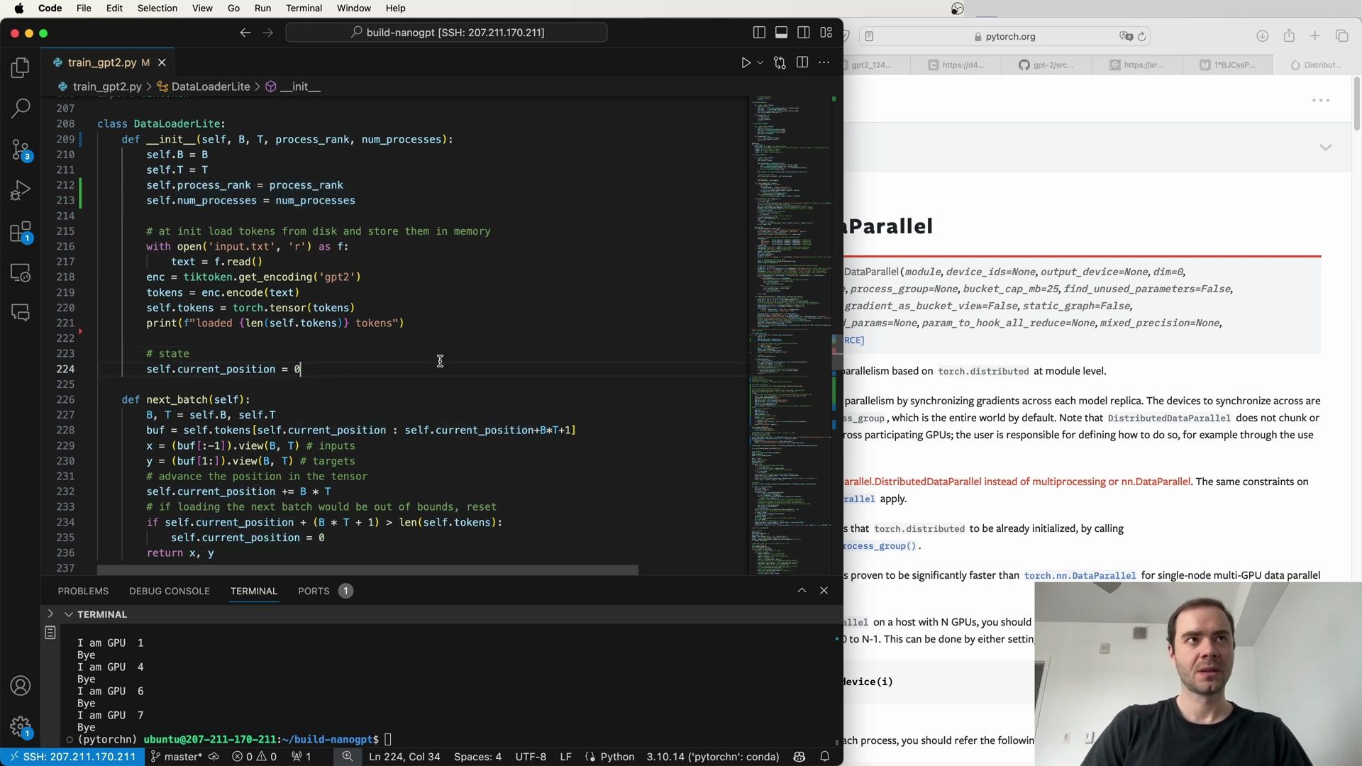
Striding Across Processes with DataLoaderLite
In the DataLoaderLite class, the stride is calculated to ensure that each process works on a different part of the dataset. The following excerpt demonstrates how the stride is implemented:
class DataLoaderLite:
    # ... other methods and initializations

    def next_batch(self):
        # Calculate the batch buffer based on the current position
        buf = self.tokens[self.current_position:self.current_position + self.B * self.T + 1]
        # Prepare input and target tensors
        x = (buf[:-1]).view(self.B, self.T)  # inputs
        y = (buf[1:]).view(self.B, self.T)  # targets
        # Advance the current position by the stride
        self.current_position += self.B * self.T * self.num_processes
        # Reset position if it exceeds the dataset length
        if self.current_position + (self.B * self.T + 1) > len(self.tokens):
            self.current_position = 0
        return x, y
By using the B, T, and num_processes variables, DataLoaderLite ensures that each process reads a unique sequence from the dataset. This is crucial for effective distributed training.
Distributed DataLoader Implementation
For efficient distributed training, it’s essential that each process works on a unique subset of the data. The DataLoaderLite class is designed to handle this by assigning a distinct chunk of the dataset to each process based on its rank. Let’s delve into the DataLoaderLite implementation and understand how it achieves this:
class DataLoaderLite:
    def __init__(self, B, T, process_rank, num_processes):
        # Initialize batch size, sequence length, process rank, and number of processes
        self.B = B
        self.T = T
        self.process_rank = process_rank
        self.num_processes = num_processes

        # Load tokens from disk and store them in memory
        with open('input.text', 'r') as f:
            text = f.read()
        enc = tokenizer.get_encoding('gpt2')
        tokens = enc.encode(text)
        self.tokens = torch.tensor(tokens)
        print(f'Process {self.process_rank} initialized with {len(self.tokens)} tokens')

    # ... other methods
The DataLoaderLite class starts by reading the entire dataset from disk and storing it in memory as a tensor of tokens. Each process is given a unique process_rank from 0 to num_processes - 1, which determines the starting point for data fetching. As training progresses, the next_batch method increments the position within the token tensor by a stride that takes into account the total number of processes, ensuring non-overlapping data segments for each process.
Device and Model Initialization
The following code snippet shows how to set up the device for training, ensuring compatibility with CUDA or MPS (Metal Performance Shaders):
if torch.cuda.is_available():
    device = 'cuda'
elif hasattr(torch.backends, 'mps') and torch.backends.mps.is_available():
    device = 'mps'
print(f'Using device: {device}')

torch.manual_seed(1337)
if torch.cuda.is_available():
    torch.cuda.manual_seed(1337)
After defining the device, we initialize the DataLoaderLite with the appropriate batch size and sequence length, as well as the rank and number of processes involved in the distributed training:
total_batch_size = 524288  # 2**19, ~0.5M, in number of tokens
B = 16  # micro batch size
T = 1024  # sequence length
assert total_batch_size % (B * T * ddp_world_size) == 0, 'Total batch size must be divisible by B * T * ddp_world_size'

train_loader = DataLoaderLite(B=B, T=T, process_rank=ddp_rank, num_processes=ddp_world_size)
Model Compilation and Learning Rate Scheduling
In distributed training, it’s vital to ensure that each process initializes the model with the same parameters. Here’s how we can compile the GPT model and set up the learning rate scheduler:
# Initialize GPT model with a specific configuration and move it to the device
model = GPT(GPTConfig(vocab_size=50304))
model.to(device)
model = torch.compile(model)

# Set the maximum and minimum learning rates and define warmup and total steps
max_lr = 6e-4
min_lr = max_lr * 0.1
warmup_steps = 10
max_steps = 50

# Define a function to calculate the learning rate based on the current step
def get_lr(step):
    if step < warmup_steps:
        # Linear warmup for the first `warmup_steps`
        return max_lr * (step + 1) / warmup_steps
    elif step >= warmup_steps:
        # After warmup, decay the learning rate using a cosine schedule
        decay_ratio = (step - warmup_steps) / (max_steps - warmup_steps)
        assert 0 <= decay_ratio <= 1
        return min_lr + (max_lr - min_lr) * 0.5 * (1.0 + math.cos(math.pi * decay_ratio))
The learning rate starts with a warm-up phase and then decays following a cosine schedule. This approach helps stabilize the training in the early phases and adjusts the learning rate dynamically based on the progress.
Parallelism and DistributedDataParallel Configuration
To achieve parallelism in distributed training, we synchronize gradients across each model replica. The DistributedDataParallel (DDP) wrapper is used to handle the parallelism at the module level. Below is a practical setup for DDP:
# DistributedDataParallel configuration
model = torch.nn.parallel.DistributedDataParallel(
    model,
    device_ids=None,
    output_device=None,
    dim=0,
    process_group=None,
    bucket_cap_mb=25,
    find_unused_parameters=False,
    gradient_as_bucket_view=False,
    static_graph=False,
    # ... additional configurations
)
Some key points about the DistributedDataParallel configuration:
- The
process_groupargument specifies the group of processes over which to synchronize gradients, with the entire world being the default. DistributedDataParalleldoes not automatically partition or chunk tensor input across GPUs.- The initialization of
torch.distributedis required by callinginit_process_group()before using DDP. - DDP can significantly outperform the traditional
torch.nn.DataParallelfor single-node, multi-GPU training.
Setting Up the Training Loop
Once the models are compiled and the learning rate scheduler is in place, the training loop can commence. Each process will independently execute the loop, processing its unique subset of data and synchronizing gradients with the others:
optimizer = model.configure_optimizers(weight_decay=0.1, learning_rate=get_lr, device=device)

for step in range(max_steps):
    # Retrieve the current learning rate
    current_lr = get_lr(step)
    # Update the optimizer's learning rate
    for param_group in optimizer.param_groups:
        param_group['lr'] = current_lr

    # Start timing the training step
    t0 = time.time()
    # Perform a training step
    # ...

    # Measure the time taken and print it
    t1 = time.time()
    if master_process:
        print(f'Training step {step} took {t1 - t0:.2f} seconds')
In this setup, we also configure the optimizer with a weight decay. The training loop fetches the learning rate for the current step, applies it to the optimizer, and executes a training step, which includes forward and backward passes and a gradient update. The timing for each step is measured to monitor the efficiency of the distributed training.
By carefully setting up the distributed data loader, device initialization, model compilation, and parallelism configuration, we can efficiently train large models like GPT in a distributed environment, leveraging multiple processes and GPUs for improved performance and scalability.
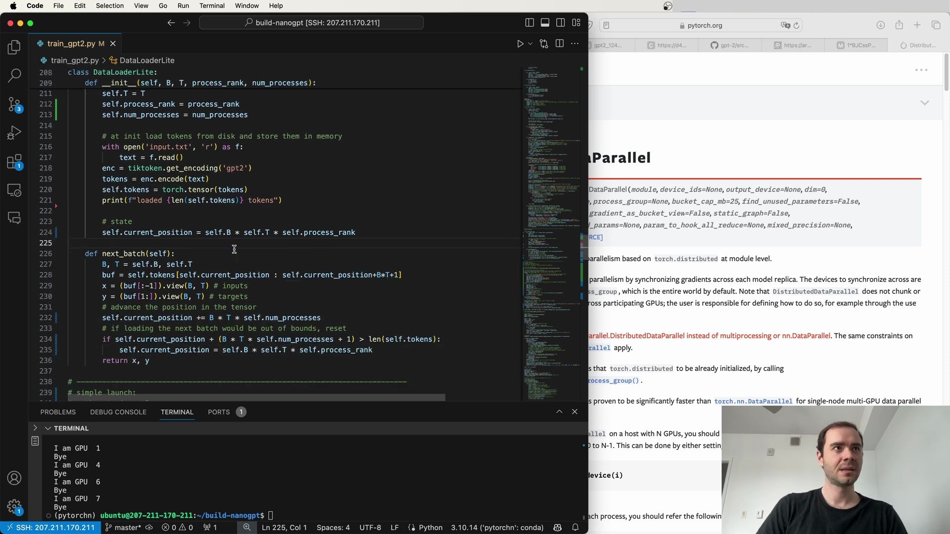
Optimizing the Training Process
When we consider the refinements within the training step, there’s a clear goal: to optimize for performance and efficiency. This involves a series of configurations and best practices, particularly when constructing the GPT model and setting up the distributed training environment.
Model Compilation and Learning Rate Adjustment
Following the initial configuration of the learning rate scheduler discussed previously, we continue with model compilation and optimization for the training loop.
# Compile the model for optimized execution
model = torch.compile(model)

# Set max and minimum learning rates and define warmup and total steps
max_lr = 6e-4
min_lr = max_lr * 0.1
warmup_steps = 10
max_steps = 500

# Optimizer setup with adjusted weight decay
optimizer = model.configure_optimizers(weight_decay=1e-5, learning_rate=6e-4, device=device)

# Commence training loop
for step in range(max_steps):
    t0 = time.time()
    optimizer.zero_grad()
    loss_accum = 0.0

    # Perform gradient accumulation steps
    for micro_step in range(grad_accum_steps):
        x, y = train_loader.next_batch()
        x, y = x.to(device), y.to(device)
        with torch.autocast(device_type=device, dtype=torch.bfloat16):
            logits, loss = model(x, y)
            # ... continue with backward pass and optimization
This snippet elaborates on the training step, with a particular focus on optimizing memory and computation through gradient accumulation and the torch.autocast context manager for mixed precision. Additionally, the optimizer is fine-tuned with a smaller weight decay, which may lead to more stable training dynamics.
Distributed Training Efficiency
To maximize efficiency in distributed training, it’s crucial to understand the nuances of the DistributedDataParallel (DDP) wrapper. Here are some essential concepts extracted from the documentation and configurations:
-
DDP Configuration: DDP wraps the model and ensures gradient synchronization across all model replicas. It does not handle tensor chunking or partitioning; this must be managed by the user.
-
Initialization: Before using DDP, the
torch.distributedframework must be initialized withinit_process_group(). -
Performance: DDP is generally faster than
torch.nn.DataParallelfor single-node, multi-GPU training. -
Model Parallelism: When using multiple GPUs, consider spawning as many processes as GPUs, minus one, to ensure each process handles a unique GPU.
# Use DistributedDataParallel for model parallelism
model = torch.nn.parallel.DistributedDataParallel(
    model,
    device_ids=None,
    output_device=None,
    dim=0,
    process_group=None,
    bucket_cap_mb=25,
    find_unused_parameters=False,
    gradient_as_bucket_view=False,
    static_graph=False,
    # ... additional configurations
)
The code block above sets up the DDP with specific configurations to optimize performance. The choice of arguments, such as bucket_cap_mb, may be adjusted based on the specifics of the training environment and model architecture.
Advanced DDP Features
DDP offers several advanced features to aid in handling uneven inputs and optimizing synchronization:
-
DDP Join Hook: Allows for training on uneven inputs by mirroring communications during forward and backward passes.
-
No Sync Context Manager: Temporarily disables gradient synchronization, which is useful for accumulating gradients over sub-steps.
# Example usage of DDP join hook and no_sync context manager
ddp = torch.nn.parallel.DistributedDataParallel(model, pg)
with ddp.no_sync():
    for input in inputs:
        ddp(input).backward()  # no sync
    ddp(another_input).backward()  # sync occurs here
In the example above, the no_sync() context manager is used to accumulate gradients locally before synchronizing them at the end of the context. This technique can help to reduce communication overhead when appropriate.
Synchronizing Across Multiple GPUs
Further details on the synchronization process provided by DDP includes:
-
Process Group: By default, the entire world (all processes) is used for synchronization unless specified otherwise.
-
Static Graphs: Set the
static_graphparameter toTrueif the graph does not change between iterations, which can improve efficiency.
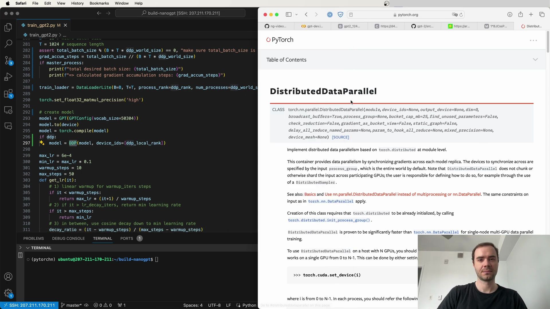
The image above illustrates the concept of distributed training and the role of DDP in managing the parallelism and synchronization necessary for efficient multi-GPU training.
Backend Initialization and Process Spawning
Finally, to establish a distributed training environment that spans multiple GPUs, the following steps are essential:
- Initialize the
torch.distributedbackend with the desired communication protocol, typically ‘nccl’ for CUDA GPUs. - Spawn the requisite number of processes, ensuring each is associated with a unique GPU.
# Backend initialization for each process
torch.distributed.init_process_group(
    backend='nccl', world_size=N, init_method='...'
)

# Associate each process with a specific GPU
torch.cuda.set_device(i)
model = DistributedDataParallel(model, device_id=[i])
In summary, efficient distributed training with the GPT model requires meticulous setup of the data loader, device initialization, model compilation, learning rate scheduling, and synchronization mechanisms. By leveraging DDP and the various features and configurations discussed here, large-scale models can be trained with improved performance and scalability.
Understanding DistributedDataParallel in Depth
In the realm of distributed training, the DistributedDataParallel (DDP) class plays a pivotal role by enabling data parallelism at the module level. It achieves this by synchronizing gradients across each model replica, but it’s worth noting that DDP does not handle tensor chunking or sharding. It’s the responsibility of the user to define how the input is partitioned, often through the use of a DistributedSampler.
import torch
from torch.nn.parallel import DistributedDataParallel as DDP

# Example of initializing a DDP object
model = ...  # assume some model
model = DDP(model, device_ids=[ddp_local_rank])
The creation of a DistributedDataParallel instance mandates that torch.distributed be already initialized by calling torch.distributed.init_process_group(). DDP has been proven to be significantly faster than torch.nn.DataParallel for single-node, multi-GPU data parallel training.
Key Properties of DistributedDataParallel:
- No Input Chunking: The input must be manually partitioned across GPUs.
- Initialization: Requires prior initialization of
torch.distributed. - Speed: Offers performance benefits over
torch.nn.DataParallel.
Best Practices for DistributedDataParallel Setup:
- Spawn as many processes as there are GPUs, ensuring each process exclusively works on a single GPU.
- Use
torch.cuda.set_device(i)to ensure that each process is associated with the correct GPU.
# Set the device for each process
torch.cuda.set_device(ddp_local_rank)
Optimizing Batch Sizes for DDP
When setting up distributed training with DDP, it’s crucial to ensure that the total batch size is divisible by the product of the number of gradient accumulation steps, the sequence length, and the world size of the DDP configuration. This requirement helps in maintaining a balanced workload across all processes.
# Assert condition for total batch size divisibility
assert total_batch_size % (B * T * ddp_world_size) == 0, "Total batch size must be divisible by B * T * ddp_world_size"
The assert statement above checks for this condition, and if it’s not met, the training process will halt, prompting the user to adjust the batch sizes accordingly.
Diving Deeper into the DDP Mechanism
The true power of DDP lies in its ability to synchronize gradients across all participating devices during the backward pass. While the forward pass remains unchanged, the backward pass in DDP is augmented with a gradient averaging step. Once the backward pass is complete on each GPU, DDP performs an all-reduce operation, averaging the gradients across all ranks.
DDP also provides efficiency by overlapping communication with computation. While the backward pass is still in progress, DDP can initiate gradient synchronization for layers that have already completed their backward computation. This overlap maximizes hardware utilization and speeds up training.
DataLoader and Training Loop Adjustments for DDP
For a model to be trained with DDP, it’s essential to configure the data loader and training loop appropriately. The following code snippet illustrates the setup of a data loader and the adjustments made to the training loop to accommodate DDP.
from torch.utils.data import DataLoader
from GPT import GPT, GPTConfig

# DataLoader setup for distributed training
train_loader = DataLoader(lite_bs=1, local_process_rank=ddp_local_rank, num_processes=ddp_world_size)

# Create and compile the model
model = GPT(GPTConfig(vocab_size=50304))
model.to(device)
model = torch.compile(model)

# Wrap the model with DDP if enabled
if ddp:
    model = DDP(model, device_ids=[ddp_local_rank])
In the training loop, the learning rate is dynamically adjusted, and gradient accumulation is handled carefully to avoid premature gradient synchronization.
# Learning rate schedule function
def get_lr(it):
    # Warmup, decay, and other lr schedule details

# Configure optimizers with weight decay and learning rate
optimizer = model.configure_optimizers(weight_decay=0.1, learning_rate=6e-4, device=device)

# Training loop with gradient accumulation
for step in range(max_steps):
    # ... training loop details, including gradient accumulation
Synchronizing Gradients with Gradient Accumulation
During training with gradient accumulation, it’s important not to synchronize gradients after every backward pass, as this would be inefficient. Instead, gradients should be accumulated locally and synchronized only at the final step. This behavior is controlled using the no_sync context manager.
# Gradient accumulation and synchronization
for step in range(max_steps):
    optimizer.zero_grad()
    loss_accum = 0.0
    for micro_step in range(grad_accum_steps):
        x, y = next(train_loader)
        x, y = x.to(device), y.to(device)
        # Forward and backward passes here
        # ...
        if micro_step == grad_accum_steps - 1:
            # Synchronize gradients on the last step
            pass  # This is where the synchronization happens
Cautionary Note on DistributedDataParallel
It’s important to note that using DistributedDataParallel in conjunction with the Distributed RPC Framework is experimental and subject to change. This means that while it can be a powerful tool, developers should be prepared for potential updates or modifications to the API.
Detailed Parameters for DistributedDataParallel
The DistributedDataParallel class accepts a range of parameters that control its behavior:
module: The module to be parallelized.device_ids: The CUDA devices for single-device modules.output_device: Device location of output for single-device CUDA modules.broadcast_buffers: Enables syncing of the module’s buffers at the beginning of the forward function.process_group: The process group used for distributed data all-reduction.bucket_cap_mb: Controls the bucket size for gradient reduction.find_unused_parameters: Identifies parameters that don’t receive gradients.gradient_as_bucket_view: When set to True, gradients will be views of the allreduce communication buckets.
# Initialization of DDP with detailed parameters
model = DDP(model, device_ids=[ddp_local_rank], broadcast_buffers=True, bucket_cap_mb=25, find_unused_parameters=False, gradient_as_bucket_view=True)
The correct use of these parameters ensures that DistributedDataParallel operates efficiently and that the gradients are handled in the most optimal fashion for the given training configuration.
Conclusion
By understanding and properly configuring DistributedDataParallel, developers can leverage the full power of distributed training, leading to faster and more efficient model training on multiple GPUs. Whether it’s synchronizing gradients, optimizing batch sizes, or dynamically adjusting learning rates, each aspect plays a crucial role in the overarching goal of scaling deep learning models.
Advanced Gradient Management with DDP
Properly managing gradients is a critical aspect of training models efficiently with DistributedDataParallel. As we continue to delve into the intricacies of DDP, we uncover that during the training loop, there are several important steps and considerations to ensure that gradients are handled correctly.
optimizer = model.configure_optimizers(warmup_tokens=warmup_tokens, final_tokens=final_tokens, weight_decay=0.1, learning_rate=6e-4, device=device)

for step in range(max_steps):
    t0 = time.time()
    optimizer.zero_grad()
    loss_accum = 0.0
    for micro_step in range(grad_accum_steps):
        x, y = next(train_loader)
        x, y = x.to(device), y.to(device)
        with torch.autocast(device_type=device, dtype=torch.bfloat16):
            logits, loss = model(x, y)
        loss = loss / grad_accum_steps  # Scale the loss for gradient accumulation
        loss_accum += loss.detach()
    loss.backward()
    norm = torch.nn.utils.clip_grad_norm_(model.parameters(), 1.0)
    lr = get_lr(step)  # Adjust learning rate dynamically
    for param_group in optimizer.param_groups:
        param_group['lr'] = lr
    optimizer.step()
    torch.cuda.synchronize()  # Ensure synchronization of GPUs
    t1 = time.time()
    tokens_processed = train_loader.b * train_loader.T * grad_accum_steps
    tokens_per_sec = tokens_processed / (t1 - t0)
Key Considerations:
- Gradient Accumulation: To handle larger batch sizes than what a single GPU can process, gradients are accumulated across multiple forward-backward passes.
- Loss Scaling: The loss must be scaled down by the number of accumulation steps to simulate averaging the gradients, as opposed to summing them.
- Learning Rate Scheduling: The learning rate is dynamically adjusted each iteration based on a predefined schedule.
- Gradient Clipping: Gradients are clipped to prevent the exploding gradient problem, ensuring stable training.
Disabling Gradient Synchronization
In certain scenarios, we may want to temporarily disable gradients synchronization across DDP processes. This can be accomplished using the no_sync context manager. This context allows gradients to be accumulated locally without immediate synchronization, which can be beneficial for efficiency.
# Example usage of no_sync context manager
with ddp.no_sync():
    for input in inputs:
        ddp(input).backward()  # Accumulate gradients without synchronization
ddp(another_input).backward()  # Outside the context, synchronize gradients
Note: It is imperative that the forward pass is included inside the no_sync context manager to ensure proper gradient accumulation.
Communication Hooks in DDP
PyTorch’s DDP also allows for the registration of user-defined communication hooks, which can be used to implement custom DDP aggregation algorithms. These hooks can be a powerful tool for trying out new distributed training ideas.
# Registering a communication hook
def my_comm_hook(state, bucket):
    # Custom communication operations here

ddp.register_comm_hook(state, my_comm_hook)
Gradient Division by World Size
The DDP framework offers a keyword argument, divide_by_initial_world_size, which controls how gradients are averaged across processes. By setting this to True, gradients are divided by the initial world size when DDP was launched. If set to False, gradients are divided by the effective world size, which accounts for the number of non-joined processes.
Parameters:
divide_by_initial_world_size(bool, optional): A flag to control the division of gradients during the backward pass. Defaults toTrue.
Monitoring Training Performance
During training, it’s useful to monitor the performance of the model. One way to do this is by calculating the number of tokens processed per second.
# Calculate tokens per second to monitor training performance
tokens_per_sec = tokens_processed / (t1 - t0)
This metric can provide insights into how efficiently the training is utilizing the available computational resources.
Problems and Debugging
When encountering issues during the setup or execution of DDP training, it’s often necessary to dive into debugging. This might involve examining the output from the training loop, checking for errors, and ensuring that the model and DDP are correctly configured.
# Debugging in a terminal
(pytorch) ubuntu@207-211-170-211:~/build-nanogpt$
Best Practices:
- Regular Checks: Continuously check for any anomalies in loss values, gradients, or performance metrics.
- Logging: Utilize logging to track the progress and state of the training loop.
- Validation: Periodically validate the model on a separate dataset to ensure learning is proceeding as expected.
In Summary
Mastering the advanced features of DistributedDataParallel can lead to more efficient and effective training of large-scale models. By carefully managing gradients, utilizing context managers like no_sync, and implementing custom communication hooks, one can tailor the training process to specific needs and potentially achieve better results. Monitoring key metrics such as tokens processed per second and employing best practices in debugging are essential for maintaining a smooth and successful training operation.
Granular Control of Gradient Synchronization
When leveraging DistributedDataParallel (DDP), it’s sometimes necessary to fine-tune the synchronization of gradients to optimize performance. An example of this is when we want to synchronize only on certain conditions. The following snippet illustrates how we can exert granular control over this feature.
# Configuration of optimizer with specific hyperparameters
optimizer = model.configure_optimizers(
    warmup_tokens=375e6,
    final_tokens=260e9,
    max_lr=6e-4,
    weight_decay=0.1,
    learning_rate=6e-4,
    device=device
)

# Training loop with granular gradient synchronization control
for step in range(max_steps):
    t0 = time.time()
    optimizer.zero_grad()
    loss_accum = 0.0
    for micro_step in range(grad_accum_steps):
        x, y = next(train_loader)
        x, y = x.to(device), y.to(device)
        with torch.autocast(device=device, dtype=torch.bfloat16):
            logits, loss = model(x, y)

        # Scale the loss to account for gradient accumulation
        loss = loss / grad_accum_steps
        loss_accum += loss.detach()

    # Only synchronize gradients on the final micro_step
    if loss_accum:
        model.require_backward_grad_sync = (micro_step == grad_accum_steps - 1)
        loss.backward()

    norm = torch.nn.utils.clip_grad_norm_(model.parameters(), 1.0)

    # Determine and set the learning rate for this iteration
    lr = get_lr(step)
    for param_group in optimizer.param_groups:
        param_group['lr'] = lr

    optimizer.step()
    torch.cuda.synchronize() # Wait for the GPU to finish work
    t1 = time.time()
    dt = t1 - t0 # Time difference in seconds
    tokens_processed += train_loader.B * train_loader.T * grad_accum_steps
In this code block:
model.require_backward_grad_syncis strategically set toTrueonly during the final iteration of the micro steps.- Gradient synchronization is disabled on all but the last micro_step within the loop, reducing the synchronization overhead.
- The final call to
loss.backward()triggers gradient synchronization across all processes.
Dynamic Gradient Synchronization
Dynamic adjustment of gradient synchronization based on specific training conditions can lead to more efficient use of computational resources. This technique is particularly handy when different parts of the training loop require different synchronization behavior.
# Training loop with dynamic gradient synchronization based on training conditions
for step in range(max_steps):
    t0 = time.time()
    optimizer.zero_grad()
    loss_accu = 0.0
    for micro_step in range(grad_accum_steps):
        x, y = next(train_loader)
        x, y = x.to(device), y.to(device)
        with torch.autocast(device_type=device, dtype=torch.bfloat16):
            logits, loss = model(x, y)

        # Scale the loss for gradient accumulation
        loss = loss / grad_accum_steps
        loss_accu += loss.detach()

    # Enable gradient synchronization only on the last micro_step
    if loss_accu != 0:
        model.require_backward_grad_sync = (micro_step == grad_accum_steps - 1)
        loss.backward()

    norm = torch.nn.utils.clip_grad_norm_(model.parameters(), 1.0)
    # Set the learning rate for the current iteration
    lr = get_lr(step)
    for param_group in optimizer.param_groups:
        param_group['lr'] = lr

    optimizer.step()
    torch.cuda.synchronize() # Ensure GPU synchronization
    t1 = time.time()
    dt = t1 - t0 # Calculate time difference for this iteration
This approach provides:
- Flexibility: Ability to toggle synchronization based on the current state or step of training.
- Efficiency: Reduction of unnecessary communication overhead during training iterations where synchronization is not required.
Direct Toggling of Backward Synchronization
Directly toggling the require_backward_grad_sync attribute can be a delicate operation and should be done with an understanding of the potential effects on the backward pass.
# Training loop with direct toggling of backward synchronization
for step in range(max_steps):
    t0 = time.time()
    optimizer.zero_grad()
    loss_accum = 0.0
    for micro_step in range(grad_accum_steps):
        x, y = next(loader)
        x, y = x.to(device), y.to(device)
        with torch.autocast(device_type=device, dtype=torch.bfloat16):
            logits, loss = model(x, y)

        # Scale loss for proper gradient accumulation
        loss = loss / grad_accum_steps
        loss_accum += loss.detach()

    if dp:
        # Toggle synchronization only on the last micro_step
        model.require_backward_grad_sync = (micro_step == grad_accum_steps - 1)
    loss.backward()

    norm = torch.nn.utils.clip_grad_norm_(model.parameters(), 1.0)
    # Adjust learning rate for this iteration
    lr = get_lr(step)
    for param_group in optimizer.param_groups:
        param_group['lr'] = lr

    optimizer.step()
    torch.cuda.synchronize() # Complete GPU tasks
    t1 = time.time()
    dt = t1 - t0 # Time taken for this iteration
In this scenario, the synchronization of gradients is controlled directly by changing the require_backward_grad_sync flag at the appropriate time within the gradient accumulation loop.
Caution: Manipulating this flag can affect the integrity of the backward pass and should be used with caution. This method is not conventional and may not be supported in future versions of PyTorch DDP.
By implementing these strategies, we ensure that the synchronization of gradients is performed only when necessary, optimizing the overall training process in a distributed environment. This leads to a more efficient use of computational resources, potentially reducing training time without compromising the quality of the model.
Fine-Tuning the Backward Pass
During training with distributed data parallelism, it’s essential to fine-tune the backward pass to ensure that gradients are synchronized effectively. The following example demonstrates how the require_backward_grad_sync variable can be toggled to control when gradients are synchronized during the backward pass.
# Set up the optimizer with model-specific configurations
optimizer = model.configure_optimizers(weight_decay=0.1, learning_rate=6e-4, device=device)

for step in range(max_steps):
    t0 = time.time()
    optimizer.zero_grad()
    loss_accum = 0.0
    for micro_step in range(grad_accum_steps):
        x, y = next(train_loader)
        x, y = x.to(device), y.to(device)
        with torch.autocast(device_type=device, dtype=torch.bfloat16):
            logits, loss = model(x, y)
        # Scale the loss for gradient accumulation
        loss = loss / grad_accum_steps
        loss_accum += loss.detach()
    if ddp:
        # Toggle synchronization only on the last micro_step
        model.require_backward_grad_sync = (micro_step == grad_accum_steps - 1)
    loss.backward()
    norm = torch.nn.utils.clip_grad_norm_(model.parameters(), 1.0)
    # Set the learning rate for the current iteration
    lr = get_lr(step)
    for param_group in optimizer.param_groups:
        param_group['lr'] = lr
    optimizer.step()
    torch.cuda.synchronize() # Ensure all GPU operations are finished before proceeding
    t1 = time.time()
    dt = t1 - t0 # Calculate the time difference for this iteration
    tokens_processed = train_loader.B * train_loader.T * grad_accum_steps
    tokens_per_sec = tokens_processed / dt
This code snippet highlights several key practices:
- Loss Scaling: To account for gradient accumulation, the loss is scaled down. This ensures the gradients correspond to the mean rather than the sum of the losses over the micro_steps.
- Synchronization Control: By setting
model.require_backward_grad_synctoTrueonly on the last micro_step, we minimize synchronization overhead. - Gradient Clipping:
torch.nn.utils.clip_grad_norm_is used to prevent exploding gradients, stabilizing training.
Handling Gradient Averaging
With distributed training, it’s not only gradients that need to be synchronized but also the loss values across different processes. The code below demonstrates how to average the loss across all processes in a distributed setting, thereby aligning the averaged gradients with the averaged loss.
# Training loop with averaging of loss across all processes in DDP
for step in range(max_steps):
    t0 = time.time()
    optimizer.zero_grad()
    loss_accum = 0.0
    for micro_step in range(grad_accum_steps):
        x, y = train_loader.next_batch()
        x, y = x.to(device), y.to(device)
        with torch.autocast(device_type=device, dtype=torch.bfloat16):
            logits, loss = model(x, y)
        # Adjust the loss based on the number of gradient accumulation steps
        loss = loss / grad_accum_steps
        loss_accum += loss.item() # Use .item() to get the actual loss value
        loss.backward()
        if model.require_backward_grad_sync == (micro_step == grad_accum_steps - 1):
            model.backward()
    norm = torch.nn.utils.clip_grad_norm_(model.parameters(), 1.0)
    # Update learning rate based on the current training step
    lr = get_lr(step)
    for param_group in optimizer.param_groups:
        param_group['lr'] = lr
    optimizer.step()
    torch.cuda.synchronize() # Sync to ensure all GPU tasks are completed
    t1 = time.time()
    dt = t1 - t0 # Duration of this training step
    items_processed = train_loader.B * (step+1) * grad_accum_steps
In this example, we observe:
- Loss Averaging: The loss is accumulated and then averaged by using
.item(), which extracts the scalar value from the tensor. - Backward Synchronization: Synchronization is explicitly invoked by checking the condition
model.require_backward_grad_sync.
Distributed Averaging of Loss
The averaging of loss is crucial for a consistent view of the model’s performance across all distributed processes. Below is an example showing how to average the loss over all distributed processes using PyTorch’s dist.all_reduce with ReduceOp.AVG.
# Training loop with distributed averaging of loss
for step in range(max_steps):
    t0 = time.time()
    optimizer.zero_grad()
    loss_accum = 0.0
    for micro_step in range(grad_accum_steps):
        x, y = train_loader.next_batch()
        x, y = x.to(device), y.to(device)
        with torch.autocast(device_type=device, dtype=torch.bfloat16):
            logits, loss = model(x, y)
        # Scale the loss to account for gradient accumulation
        loss = loss / grad_accum_steps
        loss_accum += loss.detach().item() # Note the conversion to a Python float
        loss.backward()
    if ddp:
        # Average the loss across all distributed processes
        dist.all_reduce(loss, op=dist.ReduceOp.AVG)
    norm = torch.nn.utils.clip_grad_norm_(model.parameters(), 1.0)
    # Dynamically set the learning rate for this iteration
    lr = get_lr(step)
    for param_group in optimizer.param_groups:
        param_group['lr'] = lr
    optimizer.step()
    torch.cuda.synchronize() # Complete all pending GPU operations
    t1 = time.time()
Important aspects covered in this section:
- Loss Detachment and Reduction: The loss tensor is detached and then converted to a Python float for averaging.
- Distributed Reduction:
dist.all_reduceis used to average the scalar loss across all processes, ensuring a consistent view of the loss.
By implementing the above strategies, we optimize the gradient synchronization process, which is pivotal in distributed training. This not only enhances the training efficiency but also ensures that all processes have a coherent understanding of the model’s performance, which is critical for the convergence and generalizability of the trained model.
Gradient Accumulation and Averaging
When training deep learning models, especially in a distributed setting, we often deal with gradient accumulation and averaging to handle large batches or to synchronize updates across multiple devices. This is a critical part of model optimization that ensures consistent updates and model convergence. Let’s delve into the implementation details and considerations for these techniques.
Scaling Loss for Gradient Accumulation
During the training loop, especially in the context of gradient accumulation, it’s necessary to scale the loss. This is because the gradients are added up across successive backward passes, which corresponds to summing the objective when we actually want the mean. Here’s how we can correctly scale the loss:
for step in range(max_steps):
    t0 = time.time()
    optimizer.zero_grad()
    loss_accum = 0.0
    for micro_step in range(grad_accum_steps):
        x, y = train_loader.next_batch()
        x, y = x.to(device), y.to(device)
        with torch.autocast(device_type=device, dtype=torch.bfloat16):
            logits = model(x, y)
            loss = loss_module(logits, y)
        loss = loss / grad_accum_steps  # Scale the loss for correct averaging
        loss_accum += loss.detach()
    if loss_accum != 0:
        model.require_backward_grad_sync = (micro_step == grad_accum_steps - 1)
        loss.backward()
    if ddp:
        # Distributed averaging of loss across processes
        dist.all_reduce(loss_accum, op=dist.ReduceOp.AVG)
    norm = torch.nn.utils.clip_grad_norm_(model.parameters(), 1.0)
    lr = get_lr(step)  # Set learning rate for the iteration
    for param_group in optimizer.param_groups:
        param_group['lr'] = lr
    optimizer.step()
    torch.cuda.synchronize()  # Wait for GPU to finish work
    t1 = time.time()
    dt = t1 - t0  # Time difference in seconds
    examples_per_second = train_loader.B * max_steps / dt
In the above code, notice that:
- Loss scaling is done by dividing the loss by the number of gradient accumulation steps.
- The
loss_accumvariable is used to keep track of the scaled loss across all micro-steps. - The
dist.all_reducefunction is employed to average the loss across all distributed processes when using Distributed Data Parallel (DDP).
Synchronization of Gradients
In the distributed context, it’s essential to control when gradients are synchronized across different processes:
# Disable gradient synchronizations across DDP processes
# Gradients will be accumulated on module variables, which will later be synchronized
with torch.nn.parallel.DistributedDataParallel(model, pg).no_sync():
    for input in inputs:
        model(input).backward()  # No synchronization, accumulate grads
    model(input).backward()  # Synchronize grads
The no_sync() context manager is a valuable tool to accumulate gradients locally without immediate synchronization. This is important for efficiency as it reduces the communication overhead during the majority of micro-steps.
GPT Neural Network Architecture
Let’s look at a snippet of the code that defines a block of the GPT neural network architecture, including its configuration:
class Block(nn.Module):
    def __init__(self, config):
        super().__init__()
        self.ln_1 = nn.LayerNorm(config.n_embd)
        self.attn = CausalSelfAttention(config)
        self.mlp = MLP(config)

    def forward(self, x):
        x = x + self.attn(self.ln_1(x))
        x = x + self.mlp(self.ln_2(x))
        return x

@dataclass
class GPTConfig:
    block_size: int = 1024  # Max sequence length
    vocab_size: int = 50257  # Number of tokens: BPE merges + bytes tokens + endoftext token
    n_layer: int = 12  # Number of layers
    n_head: int = 12  # Number of heads
    n_embd: int = 768  # Embedding dimension

class GPT(nn.Module):
    def __init__(self, config):
        super().__init__()
        self.config = config
        self.transformer = nn.ModuleDict({
            "wte": nn.Embedding(config.vocab_size, config.n_embd),
            "wpe": nn.Embedding(config.block_size, config.n_embd),
            "h": nn.ModuleList([Block(config) for _ in range(config.n_layer)]),
            "ln_f": nn.LayerNorm(config.n_embd),
        })
        self.lm_head = nn.Linear(config.n_embd, config.vocab_size, bias=False)
In this architecture:
Blockclass represents a single transformer block, which includes layer normalization, self-attention, and a multilayer perceptron (MLP).GPTConfigis a dataclass that holds the configuration parameters for the model.GPTclass is the main model that encapsulates the transformer blocks and the final linear layer for language modeling.
DataLoader Simplification
A lightweight version of the DataLoader can be implemented to streamline the process of feeding data into the model:
class DataLoaderLite:
    def __init__(self, B, T, process_rank, num_processes):
        tokens = enc.encode(text)
        tokens = torch.tensor(tokens)
        self.tokens = tokens
        print(f"DataLoader initialized with batch size {B} and sequence length {T}")
In this DataLoaderLite, the constructor takes basic parameters such as batch size (B) and sequence length (T) and prepares the tokenized text for training.
Learning Rate Scheduling
The learning rate is dynamically adjusted throughout the training process using a cosine decay schedule that takes into account warmup steps and the maximum number of steps:
def get_lr(t):
    # Cosine decay of learning rate after warmup
    decay_ratio = (t - warmup_steps) / (max_steps - warmup_steps)
    assert 0 <= decay_ratio <= 1
    coeff = 0.5 * (1.0 + math.cos(math.pi * decay_ratio))
    return min_lr + coeff * (max_lr - min_lr)
Here, get_lr function calculates the learning rate at a given training step t, providing a smooth transition from a higher learning rate to a lower one, ensuring stable training.
In conclusion, by scaling the loss for gradient accumulation, managing synchronization of gradients in a distributed context, understanding the GPT architecture, simplifying data loading, and scheduling the learning rate, we establish a robust foundation for training large-scale language models effectively.
Handling Gradient Accumulation
In the process of training our GPT-2 model, we need to be meticulous in handling the gradient accumulation. This is because the gradients get aggregated across successive backward passes, which, if not managed properly, could skew the objective from a mean to a sum. To counter this, we scale the loss accordingly:
loss = loss / grad_accum_steps
loss_accum += loss.detach()
Here, loss is divided by grad_accum_steps, ensuring that the accumulation translates to an average, rather than a sum. This is crucial for maintaining the integrity of the training objective.
Distributed Data Parallel (DDP) Considerations
When in a distributed setting (denoted by ddp), additional steps are taken to manage the gradients across multiple devices. We synchronize only on the last accumulation step and then perform an all-reduce operation to average the loss across processes:
if ddp:
    model.require_backward_grad_sync = (micro_step == grad_accum_steps - 1)
    loss.backward()

if ddp:
    dist.all_reduce(loss_accum, op=dist.ReduceOp.AVG)
The dist.all_reduce function is instrumental here, as it averages the accumulated loss across all nodes participating in the training. This ensures a consistent and fair contribution of gradients from all nodes.
Gradient Clipping and Learning Rate Adjustment
To maintain stability during training, clipping the gradients is a common practice. It prevents the model from taking overly large steps during optimization, which could lead to divergent behavior:
norm = torch.nn.utils.clip_grad_norm_(model.parameters(), 1.0)
We also dynamically adjust the learning rate for each iteration. This is crucial for the model to learn effectively:
lr = get_lr(step)
for param_group in optimizer.param_groups:
    param_group['lr'] = lr
optimizer.step()
The function get_lr calculates the learning rate based on the current step, and the learning rate is applied across all parameter groups of the optimizer.
Synchronizing and Measuring Performance
After performing an optimizer step, we ensure that all GPU work is finished before proceeding. This is achieved using torch.cuda.synchronize(). We also measure the time taken for each step and calculate the processing speed in tokens per second:
torch.cuda.synchronize() # wait for the GPU to finish work
t1 = time.time()
dt = t1 - t0 # time difference in seconds
tokens_processed = train_loader.B * train_loader.T * grad_accum_steps * ddp_world_size
tokens_per_sec = tokens_processed / dt
If running on the master process, we print out the current step, loss, learning rate, gradient norm, and time taken to process:
if master_process:
    print(f'step: {step:4d} | loss: {loss_accum.item():.6f} | lr {lr:.4e} | norm: {norm:.4f} | dt: {dt:.4f}')
This information is crucial for monitoring the training progress and for debugging purposes.
Learning Rate Scheduler
The learning rate scheduler plays a pivotal role in controlling the learning rate throughout the training process. A combination of linear warmup and cosine decay is used:
def get_lr(t):
    if t < warmup_steps:
        # Linear warmup
        return min_lr + t * (max_lr - min_lr) / warmup_steps
    if t > max_steps:
        # Minimum learning rate after decay
        return min_lr
    # Cosine decay to the minimum learning rate
    decay_ratio = (t - warmup_steps) / (max_steps - warm_step)
    assert 0 <= decay_ratio <= 1
    coeff = 0.5 * (1.0 + math.cos(math.pi * decay_ratio))
    return min_lr + coeff * (max_lr - min_lr)
This schedule ensures that the learning rate starts with a linear warmup, preventing the model from taking too large steps in the initial phase. After the warmup, the learning rate gradually decays following a cosine curve, which helps in settling into a better local minimum towards the end of training.
Final Debugging and Launching
Before we set the training into motion, it’s essential to make sure that the process group is properly destroyed upon completion. This is courteous to the underlying communication library (e.g., NCCL) and ensures that it does not raise any complaints when we exit the training script:
# Additional code for cleanup (not shown) would go here to destroy the process group
With these settings tuned and the debugging complete, we are ready to launch the script and monitor the output. The script’s output will provide real-time feedback on the training process, including performance metrics and the current state of the model’s optimization.
In the script, you might observe sections like:
# prefix tokens
model.eval()
num_return_sequences = 5
This is typically used for inference and to generate multiple sequences from the model, showcasing the model’s ability to predict and continue text based on the given prefix tokens.
By meticulously fine-tuning the training process through gradient scaling, distributed synchronization, learning rate scheduling, and proper debugging, we are setting our GPT-2 model on a course to effectively learn from the data and, hopefully, achieve impressive results in natural language understanding and generation tasks.
Optimizing the Learning Rate Schedule
Optimizing the learning rate is critical for the efficient training of neural networks. Our training script includes a function get_lr which adjusts the learning rate based on the iteration step. This function employs a linear warmup at the start of training followed by a cosine decay. Below is the updated function which handles the learning rate adjustment:
def get_lr(it):
    # 1) linear warmup for warmup_steps
    if it < warmup_steps:
        return min_lr + (it+1) / warmup_steps * (max_lr - min_lr)
    # 2) if it > lr_decay_iters, return min learning rate
    if it > max_steps:
        return min_lr
    # 3) in between, use cosine decay down to min learning rate
    decay_ratio = (it - warmup_steps) / (max_steps - warmup_steps)
    assert decay_ratio >= 0
    coeff = 0.5 * (1.0 + math.cos(math.pi * decay_ratio)) # coeff starts at 1 and goes to 0
    return min_lr + coeff * (max_lr - min_lr)
The get_lr function is invoked at each step to calculate the current learning rate, enabling the optimizer to adjust its parameters accordingly. The code snippet below shows the optimizer being configured and used in a loop that processes batches from the train_loader:
# Configure the optimizer with weight decay and initial learning rate
optimizer = raw_model.configure_optimizers(weight_decay=0.1, learning_rate=6e-4, device=device)

# Execute the training steps
for step in range(max_steps):
    t0 = time.time()
    optimizer.zero_grad()
    loss_accum = 0.0
    for micro_step in range(grad_accum_steps):
        x, y = train_loader.next_batch()
During the optimization process, various parameters are printed to the terminal, providing insights into the training progress. For instance, the script outputs the current step, loss, learning rate, gradient norm, time difference, and tokens processed per second:
step    loss    dt     tok/sec
0       7.906787        0.956973
...
9       7.008665        0.451130
These metrics demonstrate the performance of the training process, with the tok/sec representing the impressive rate of 1.5 million tokens processed per second.
Distributed Training Considerations
Distributed training introduces the need for special consideration regarding gradient accumulation and synchronization. When employing DistributedDataParallel (DDP), we utilize the no_sync context manager to disable gradient synchronizations across DDP processes, accumulating gradients on module variables, which are later synchronized:
torch.nn.parallel.DistributedDataParallel(model, pg)
with no_sync():
    for input in inputs:
        output = model(input)
        output.loss.backward()  # no synchronization, accumulate grads
This approach allows us to efficiently train with multiple GPUs, only synchronizing gradients when necessary.
Fine-Tuning the Optimization Loop
When fine-tuning the optimization loop, we adjust various training parameters, such as the maximum learning rate, warmup steps, and maximum steps:
max_lr = max_lr * 0.1
warmup_steps = 10
max_steps = 50

# Learning rate schedule is defined similarly as before
def get_lr(it):
    # warmup and decay logic as defined previously
    ...
The optimization loop is then executed with these updated parameters, and the training metrics are logged as follows:
for step in range(max_steps):
    t0 = time.time()
    optimizer.zero_grad()
    # Training logic
    ...

# Terminal output
step 30 | loss: 5.518186 | lr 3.0000e-04 | dt: 356.84ms | tok/sec: 1469255.70
...
step 39 | loss: 5.517982 | lr 3.0000e-04 | dt: 358.34ms | tok/sec: 1461570.49
These logs provide real-time feedback on the training process, indicating the efficiency of the model in processing a large number of tokens per second.
Adjusting for DDP Model Configuration
When transitioning from a standard model to a DDP model, it is necessary to adjust the way optimizers are configured:
# Originally it was model.configure_optimizers(...)
# Now it becomes:
optimizer = raw_model.configure_optimizers(weight_decay=0.1, learning_rate=6e-4, device=device)
Here, raw_model represents the original model before it was wrapped with DDP functionality. This adjustment ensures that the optimizer is configured correctly for the underlying model, irrespective of the DDP wrapper.
By carefully fine-tuning these training aspects, we can achieve a high level of efficiency and performance in our GPT-2 model’s training routine. This fine-grained control over training parameters allows us to navigate the complexities of large-scale language model training while maximizing the utilization of available computational resources.
Configuring Distributed Training
When setting up distributed training using PyTorch’s DistributedDataParallel (DDP), specific patterns must be followed to ensure that the model and data are correctly distributed across the available GPUs. Here is an example of how to modify the training script to support distributed training:
if torch.cuda.is_available():
    torch.cuda.manual_seed_all(42)

total_batch_size = 524288 # 2**19, ~0.5M, in number of tokens
B = 16 # micro batch size
T = 1024 # sequence length
assert total_batch_size % (B * T * ddp_world_size) == 0, "Total batch size must be divisible by the product of B, T, and the world size."

train_loader = DataLoaderLite(B=B, T=T, process_rank=ddp_rank, num_processes=ddp_world_size)
torch.set_float32_matmul_precision('high')

# create model
model = GPT(GPTConfig(vocab_size=50304))
model.to(device)
model = torch.compile(model)

if ddp:
    model = DDP(model, device_ids=[ddp_local_rank])
    raw_model = model.module if ddp else model # always contains the 'raw' unwrapped model
The DataLoaderLite is initialized with the batch size B, sequence length T, rank of the process, and the total number of processes participating in the training. It is crucial to set the random seed for reproducibility in distributed settings, and the batch size must be divisible by the product of B, T, and the world size to ensure even distribution of the workload.
Adjusting Learning Rate and Model Parameters
The following code sets up the learning rate schedule and model parameters, which are important for controlling the training process:
max_lr = 6e-4
min_lr = max_lr * 0.1
warmup_steps = 10
max_steps = 50

def get_lr(it):
    # 1) linear warmup for warmup_iters steps
    if it < warmup_steps:
        return max_lr * (it / warmup_steps)
    # 2) cosine decay to min_lr for the remaining
    else:
        dt = (it - warmup_steps) / (max_steps - warmup_steps)
        return min_lr + 0.5 * (max_lr - min_lr) * (1 + cos(pi * dt))
This script uses a linear warmup followed by a cosine decay for the learning rate. The learning rate begins with a linear increase from 0 to max_lr during warmup_steps and then follows a cosine decay to min_lr.
Output During Training
While training, the terminal prints out the progress with the current step, loss, learning rate, gradient norm, time difference, and tokens processed per second as shown below:
step 30 loss: 5.518186 lr 3.0000e-04 norm: 0.2512 dt: 356.84ms tok/sec: 14692550.70
[... repeated lines with similar step, loss, lr, norm, dt, and tok/sec values ...]
This output provides immediate feedback on the performance and progression of the model during training.
Optimizer Configuration in DDP
In distributed training, the optimizer is a critical component that needs to be configured correctly. The training script configures the optimizer as follows:
grad_accum_steps = total_batch_size // (B * T * dp_world_size)
if master_process():
    print(f"total desired batch size: {total_batch_size}")
    print(f"actual train batch size: {B // grad_accum_steps}")

# Configure optimizers
class GPT(nn.Module):
    def configure_optimizers(self, weight_decay, learning_rate, device):
        # Create AdamW optimizer and use the fused version if it is available
        fused_adam_available = 'fused_adam' in inspect.getmembers(torch.optim.AdamW)
        use_fused = fused_adam_available and 'cuda' in device
        if mast_process:
            print(f"Using fused AdamW: {use_fused}")
Within the GPT class, the configure_optimizers method determines whether to use a fused version of the AdamW optimizer, which can offer performance benefits on certain hardware. The script checks for the availability of fused_adam and decides whether to use it based on the device type.
DataLoader and Gradient Accumulation
The DataLoaderLite is tailored for distributed training and works with the training loop to handle data batching:
class DataLoaderLite:
    def __init__(self, B, T, process_rank, num_processes):
        self.tokens = torch.tensor(tokens)
        # other initialization code
The next_batch method from DataLoaderLite is used to fetch the next batch of data. It is important to note that in distributed training, each process will fetch its own subset of the data.
Gradient accumulation is a technique used to effectively increase the batch size without requiring more memory. The training script accumulates gradients over multiple steps before updating the model parameters:
for input in inputs:
    with model.no_sync(): # no synchronization, accumulate grads
        output = model(input)
        loss = loss_fn(output, target)
        loss.backward() # no synchronization, accumulate grads
    optimizer.step() # synchronize grads
The no_sync context manager is used to disable gradient synchronization across DDP processes, allowing for gradient accumulation within each process. This is essential for effectively utilizing multiple GPUs when the desired batch size exceeds the memory capacity of a single GPU.
Debugging and Problem Solving
During distributed training, it is common to encounter issues that require debugging. The training script may include debugging statements or logs to identify and resolve problems. For instance, differences in the loss values or learning rates across different training runs can be insightful for debugging.
# Debugging output
PROBLEMS
DEBUG CONSOLE
TERMINAL
PORTS
> TERMINAL
[=========================] 100% 8550.2696/8550.2696
Such debugging information can help to verify that the training is proceeding as expected and allows for the quick identification of issues related to data loading, model configuration, or other aspects of the training loop.
By integrating these components and carefully configuring the training parameters, the script enables robust and efficient distributed training for large language models like GPT-2. The use of DDP and gradient accumulation techniques ensures that the model can be trained on a large scale, taking advantage of multiple GPUs to process vast amounts of data.
Enhancing the DataLoader for Effective Batching
To facilitate distributed training, the DataLoaderLite class is crucial for managing and loading the dataset efficiently. It is responsible for ensuring that each process receives a unique subset of the data, which is an essential aspect of distributed training. Here’s an enhanced version of the DataLoaderLite to handle these tasks:
class DataLoaderLite:
    def __init__(self, B, L, T, process_rank, num_processes):
        self.B = B
        self.L = L
        self.T = T
        self.tokens = torch.tensor(tokens)  # Tokens are loaded here
        self.num_processes = num_processes
        self.process_rank = process_rank
        self.current_position = self.B * self.L * self.T * self.process_rank
        print(f'Loaded {len(self.tokens)} tokens')

    def next_batch(self):
        B, T = self.B, self.T
        buf = self.tokens[self.current_position : self.current_position + B * T + 1]
        x = buf[:-1].view(B, T)  # The input tokens
        y = buf[1:].view(B, T)   # The target tokens
        # Move the current position forward
        self.current_position += B * T * self.num_processes
        # Reset position if the next batch would be out of bounds
        if self.current_position + (B * T * self.num_processes + 1) > len(self.tokens):
            self.current_position = self.B * self.T * self.process_rank
        return x, y
In the above code, the initialization of DataLoaderLite takes in the batch size B, the number of lookahead tokens L, the sequence length T, the rank of the process (process_rank), and the total number of processes (num_processes). The next_batch method is used to fetch the next batch of input and target tokens, with careful handling of the current position within the dataset to ensure that the data is not reused inadvertently, which could lead to overfitting.
Terminal Output for Monitoring Training Progress
During the training process, it is essential to have visibility into how the model is performing. Here is an example of what the terminal output might look like, providing key metrics after each training step:
step 0  loss: 9.506379 lr 1.00000e-05 norm: 297.5145 dt: 29541.801ms t/tok/sec: 171747.32
step 1  loss: 9.629933 lr 1.00000e-05 norm: 9.3778 dt: 355.68ms t/tok/sec: 1417072.68
step 2  loss: 9.506729 lr 1.00000e-05 norm: 9.3779 dt: 355.48ms t/tok/sec: 1417827.64
...
step 19 loss: 6.174975 lr 1.00000e-05 norm: 9.3778 dt: 355.48ms t/tok/sec: 1417827.60
This output is crucial for understanding the model’s learning trajectory, as it includes the loss at each step, the learning rate (lr), the norm of the gradients (norm), the time taken for the step (dt), and the throughput in terms of tokens processed per second (t/tok/sec). Monitoring these metrics can help diagnose training issues such as exploding or vanishing gradients, slow learning rates, or bottlenecks in data processing.
Implementing Gradient Accumulation with no_sync
Gradient accumulation is a strategy used to effectively increase the batch size for training without exceeding the memory capacity of the GPUs. This technique involves accumulating gradients over multiple steps before performing an optimization step. The no_sync context manager in PyTorch’s DistributedDataParallel is used to facilitate this process:
for input in inputs:
    with model.no_sync():  # Do not synchronize gradients
        output = model(input)
        loss = loss_fn(output, target)
        loss.backward()  # Accumulate gradients locally
    optimizer.step()  # Synchronize and update model parameters
The no_sync context ensures that during the backward pass, the gradients are not synchronized across different processes. Once the gradients have been accumulated to a sufficient amount, optimizer.step() is called to update the model parameters, and at this point, gradients are synchronized.
Device Auto-detection and DDP Configuration
In a distributed training environment, it is important to auto-detect and set the appropriate device for each process. Below is an example of how device auto-detection can be implemented along with some DDP configuration:
# Attempt to autodetect the device
if torch.cuda.is_available():
    device = 'cuda'
elif hasattr(torch.backends, 'mps') and torch.backends.mps.is_available():
    device = 'mps'
print(f'using device: {device}')

torch.manual_seed(1337)
if torch.cuda.is_available():
    torch.cuda.manual_seed(1337)

# ... DDP setup ...

assert total_batch_size % (B * T * ddp_world_size) == 0, 'make sure total_batch_size is divisible by B * T * ddp_world_size'
if master_process():
    print(f'calculated desired batch size: {total_batch_size}')
    print(f'calculated gradient accumulation steps: {grad_accum_steps}')

train_loader = DataLoaderLite(B=B, T=T, process_rank=ddp_rank, num_processes=ddp_world_size)
The script first checks if CUDA is available and sets the device to ‘cuda’ if so. If CUDA is not available but the Metal Performance Shaders (MPS) backend is available on macOS, it sets the device to ‘mps’. It sets a manual seed for reproducibility and checks that the total batch size is divisible by the product of batch size B, sequence length T, and the world size of the distributed processes. If the process is the master process, it prints out the calculated desired batch size and the number of gradient accumulation steps.
Dataset Considerations for GPT-2 and GPT-3 Training
The choice of datasets is critical for training large language models like GPT-2 and GPT-3. The datasets used for GPT-3 training as listed in the paper are as follows:
- Common Crawl (filtered): 410 billion tokens, 60% weight in training mix
- WebText2: 19 billion tokens, 22% weight
- Books1: 12 billion tokens, 8% weight
- Books2: 55 billion tokens, 8% weight
- Wikipedia: 3 billion tokens, 3% weight
The weights in the training mix indicate the fraction of examples during training that come from each dataset. This intentional weighting is not proportional to the size of the dataset, which can lead to certain datasets being seen more frequently during training. Moreover, to prevent contamination of the model’s knowledge with the development or test sets, efforts were made to remove any overlaps with the benchmarks used to evaluate GPT-3.
Deduplication and Data Cleaning
Deduplication and data cleaning are essential steps to improve the quality of the datasets used for training language models. Training on deduplicated data makes models better by improving training compute efficiency and reducing the amount of data memorized from the training data. Here is an outline of the deduplication process used for creating the SlimPajama dataset from the RedPajama dataset:
- Deduplication Method: MinHashLSH with a Jaccard similarity threshold of 0.5
- Pre-processing: Removal of punctuation, consecutive spaces, numbers, leading/trailing escape characters
- Result: 49.6% of bytes pruned, resulting in a 627 billion token SlimPajama dataset
This deduplication was performed both within and between datasets, ensuring that the training data is as unique and diverse as possible, thereby increasing the robustness and generalization of the resulting language model.
The careful curation and processing of datasets play a pivotal role in training effective and efficient language models. By addressing the challenges of distributed training, monitoring progress, auto-detecting devices, and preparing high-quality datasets, researchers can push the boundaries of what’s possible with large language models like GPT-2 and GPT-3.
Dataset Diversity and Quality in LLM Training
When training LLMs, not all datasets are created equal. The quality and diversity of training data can significantly affect the model’s performance across various tasks.
Fine-Tuning Dataset Composition
In addition to the datasets previously mentioned, such as the Common Crawl and others that are standard in LLM training, some datasets are processed differently. These include GitHub, Books, Archive, Wikipedia, and Stack Exchange. Each dataset contributes unique content and style to the training data, helping to create models that can handle a wide range of language tasks.
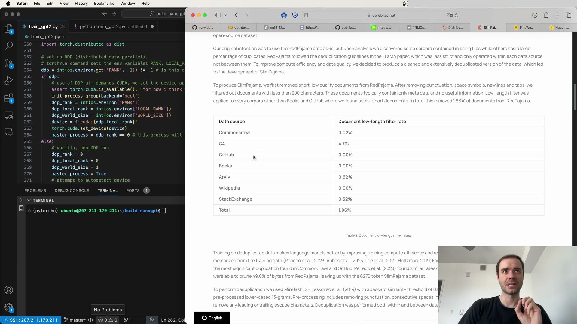
The FineWeb dataset is a recent attempt to collect high-quality Common Crawl data, filtering it down to 15 trillion tokens. High-quality datasets like FineWeb are vital for training state-of-the-art language models, and they go into significant detail about how the data was processed, which is crucial for replication and understanding the data quality.
The Creation of SlimPajama Dataset
The RedPajama dataset initially intended for use in LLM training had its share of issues, such as missing files and duplicates. The deduplication process followed the guidelines from the LLAMa paper, but it was found that these guidelines were not strict enough as they only operated within each data source, not between them. This led to the creation of the SlimPajama dataset.
Steps to Enhance Data Quality
- Initial Cleaning: Short, low-quality documents were removed from the RedPajama dataset, including those with fewer than 200 characters, which often contained only metadata without useful information.
-
Document Filtering: Application of a low-length filter to each corpus, with the exception of Books and GitHub, where shorter documents were considered useful.
Document low-length filter rates:
- Common Crawl: 0.02%
- C4: 4.7%
- GitHub: 0.00%
- Books: 0.00%
- ArXiv: 0.62%
- Wikipedia: 0.00%
- StackExchange: 0.32%
- Total: 1.86%
- Deduplication: Utilizing MinHashLSH with a Jaccard similarity threshold of 0.5, the deduplication process was performed both within and across data sources after pre-processing, which involved removing punctuation, consecutive spaces, and any leading or trailing escape characters.
The outcome of this extensive deduplication and cleaning was a 627 billion token SlimPajama dataset, which pruned 49.6% of bytes from the original RedPajama dataset.
Introducing FineWeb Dataset
Following the example of detailed dataset curation, the FineWeb dataset was introduced. It is a large-scale dataset derived from 96 CommonCrawl snapshots, encompassing over 15 trillion tokens.
Authors and Affiliations:
- Guilherme Penedo, Hynek Křížek, Loubna Ben Allal, Anton Lozhkov, Colin Raffel, Leandro Werra, Thomas Wolf
- HuggingFace
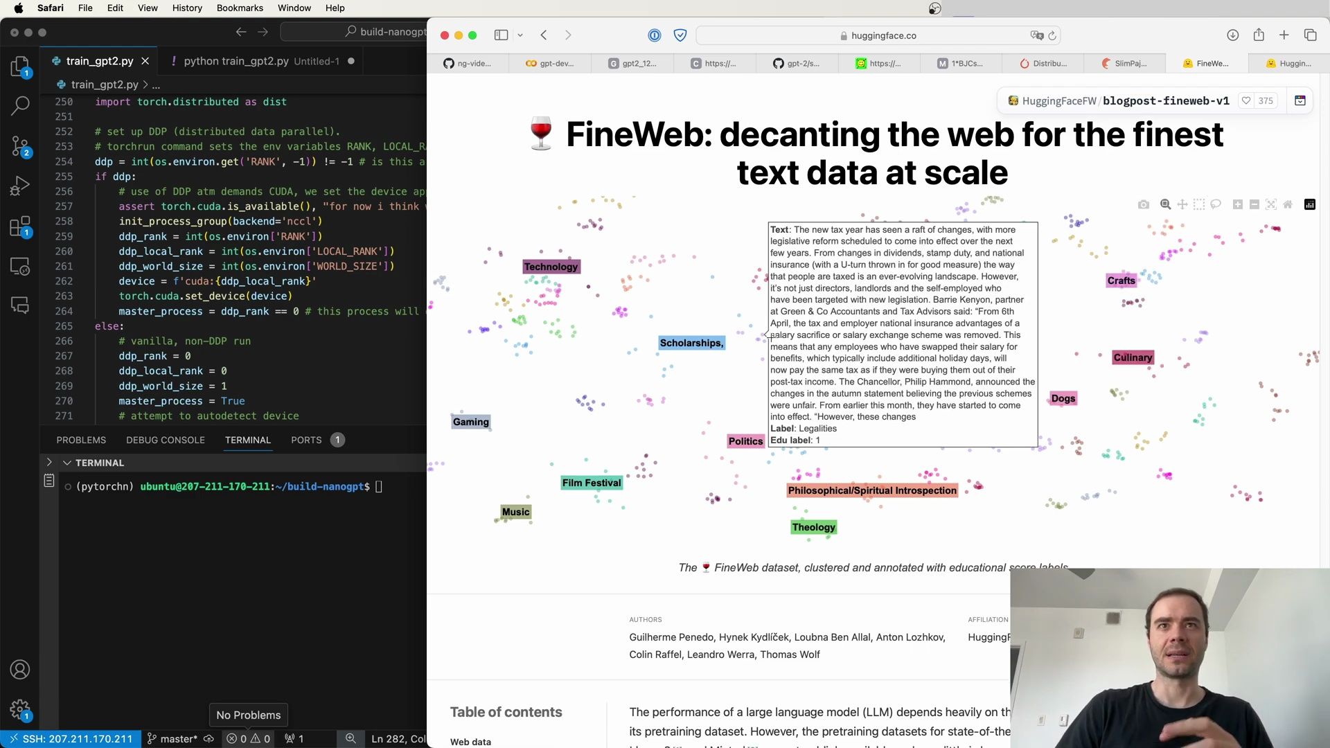
FineWeb’s Contributions
- FineWeb-Edu: A subset of FineWeb, which is curated for educational value. It comes in two sizes: 1.1 trillion tokens (very high educational content) and 5.4 trillion tokens (high educational content).
- Detailed Documentation: FineWeb’s creation process, including deduplication and filtering strategies, is meticulously documented to advance open understanding of LLM training.
The FineWeb-Edu Subset
Hugging Face’s FineWeb-Edu subset aims to filter the Common Crawl into very high-quality educational content. It is a significant contribution that provides 1.3 trillion tokens of educational content and 5.4 trillion tokens of high educational content.
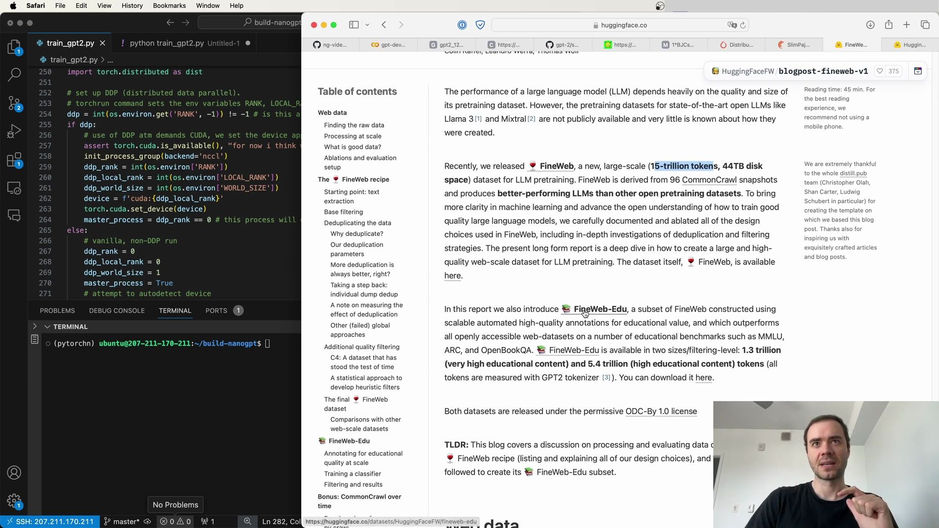
This educational subset is instrumental in training models that excel in educational benchmarks, reflecting the growing need for specialized datasets in LLM training.
Distributed Data Parallel (DDP) Configuration
Properly setting up DDP is essential for effective and efficient distributed training. The device must be auto-detected and set appropriately for each process in the distributed environment.
import torch.distributed as dist

# set up DDP (distributed data parallel).
torch.distributed.init_process_group(backend='nccl')
ddp_rank = int(os.environ.get('RANK', -1)) == -1  # is this a standalone run?
if ddp_rank:
    # Use of DDP demands CUDA, set the device accordingly
    assert torch.cuda.is_available()
    dist.init_process_group(backend='nccl')
    ddp_rank = int(os.environ.get('RANK'))
    ddp_local_rank = int(os.environ.get('LOCAL_RANK'))
    ddp_world_size = int(os.environ.get('WORLD_SIZE'))
    device = f'cuda:{ddp_local_rank}'
    torch.cuda.set_device(device)
    master_process = ddp_rank == 0  # This process will coordinate
else:
    # Vanilla, non-DDP run
    ddp_rank = 0
    ddp_local_rank = 0
    ddp_world_size = 1
    master_process = True
    # Attempt to autodetect device
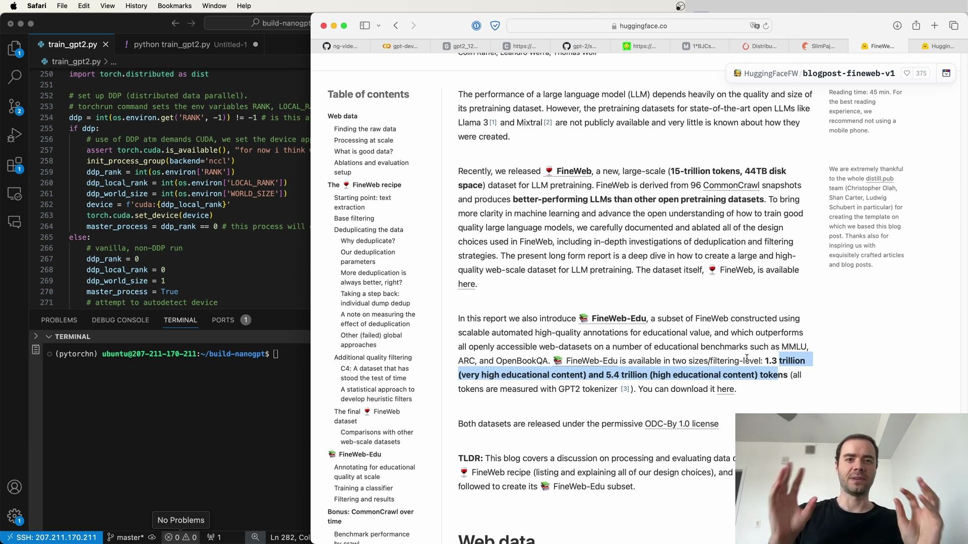
The above code snippet showcases how the DDP setup is initialized, ensuring each process is correctly configured to utilize the GPU when available, or fall back to a standalone run otherwise.
Processing Web Data at Scale
Processing web data at scale is challenging due to the sheer size involved. For the FineWeb dataset, this required a modular, scalable codebase that allowed for quick iterations and parallelized workloads.
Key points on processing at scale:
- Developed datatrove, an open-source data processing library.
- Enabled filtering and deduplication on thousands of CPU cores.
- Provided clear insights into the data.
Determining what constitutes ‘good data’ is a primary concern when creating datasets for LLM pretraining. The use of open-source libraries, such as trafilatura for text extraction from WARC files, was found to be more effective than using WET files. This decision resulted in a dataset with fewer unnecessary page boilerplates and higher quality for training LLMs.
Harnessing Educational Content for LLM Training
The importance of specialized datasets for LLM training cannot be overstated, especially when it comes to educational content. The FineWeb-Edu subset, with its 1.3 trillion tokens of the finest educational data the web has to offer, is a testament to this focus. The creators of this dataset have shown that training on educational content significantly improves performance on related metrics.
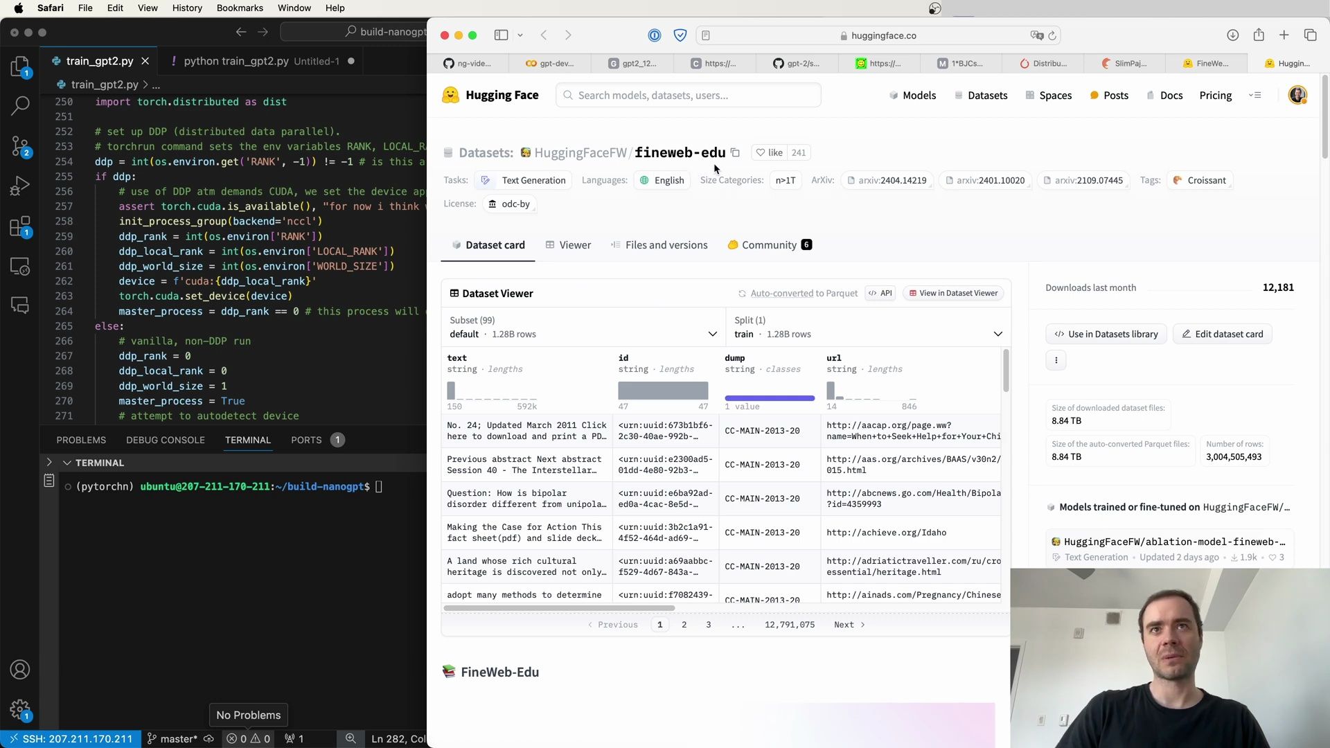
To facilitate experimentation and enable a broader range of researchers to work with this data, a 10 billion tokens subset has been made available. This manageable portion of the FineWeb-Edu dataset allows for efficient training that can closely approach the performance of models like GPT-2 without the computational overhead of processing trillions of tokens.
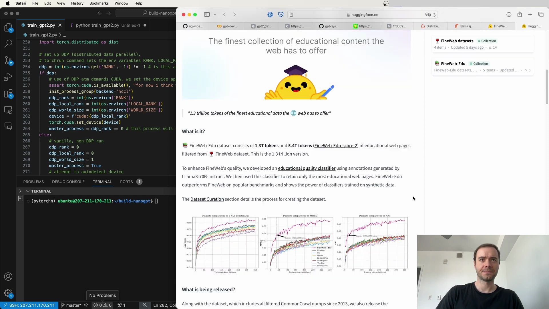
Sampling the FineWeb-Edu Dataset
When working with such a large dataset, it’s often necessary to create smaller, more manageable samples. For the FineWeb-Edu dataset, the following sample versions have been provided:
- sample-350BT: A subset randomly sampled from the whole dataset of around 350B gpt2 tokens.
- sample-100BT: A subset randomly sampled from the whole dataset of around 100B gpt2 tokens.
- sample-10BT: A subset randomly sampled from the whole dataset of around 10B gpt2 tokens.
The sample-10BT was sampled from sample-100BT, which in turn was sampled from sample-350BT. These subsets provide flexibility for researchers with varying compute resources.
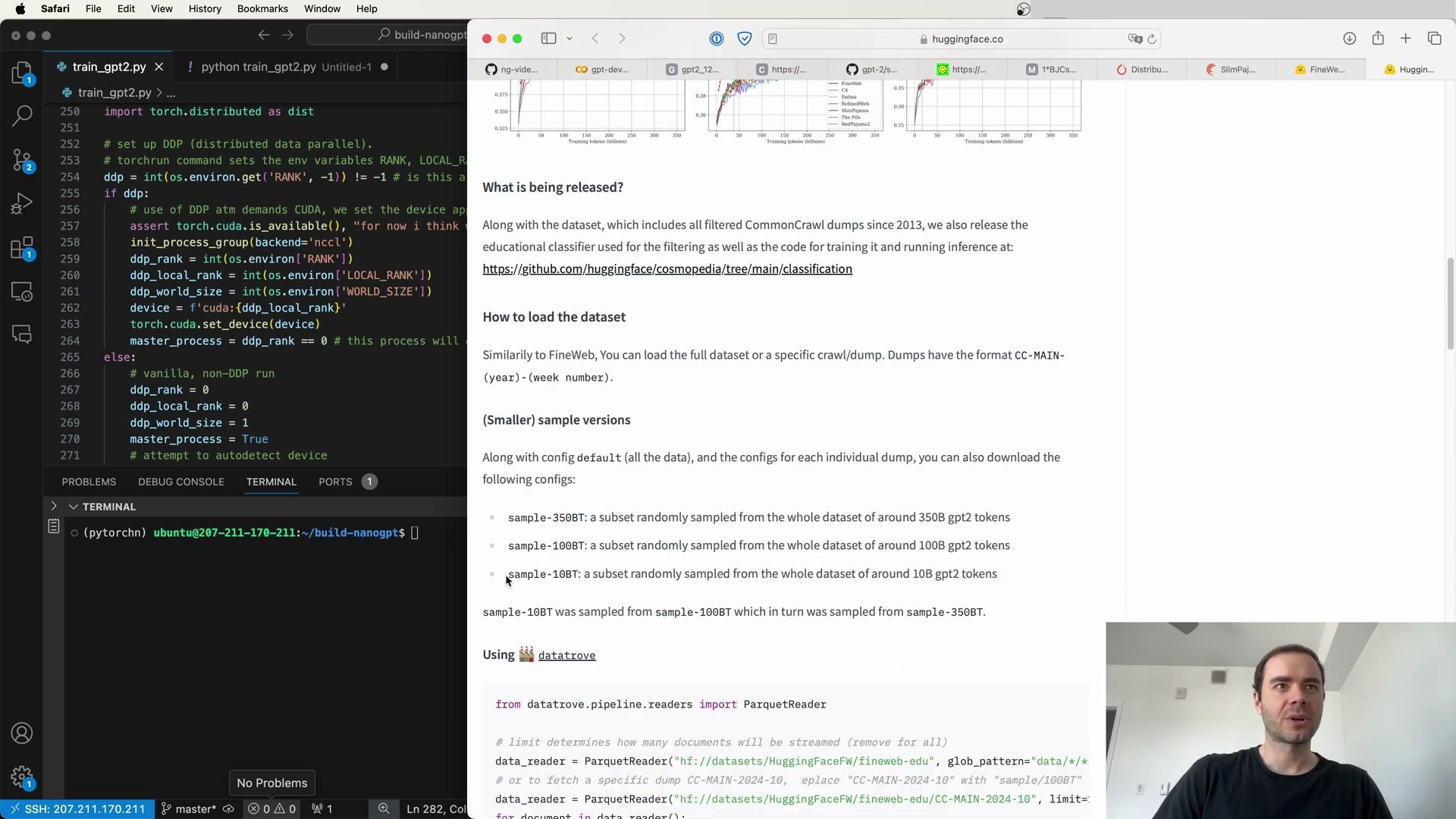
Accessing and Utilizing the Data
Hugging Face has provided convenient tools to access and work with the FineWeb-Edu dataset, including the educational classifier used for the filtering process. These resources are available in a publicly accessible GitHub repository:
- Educational Classifier and Training Code: HuggingFace Cosmopedia Classification
The dataset itself can be loaded in full or as specific crawls/dumps, with the format CC-MAIN-(year)-(week number).
Distributed Data Parallel Setup
Working with such extensive datasets requires a robust setup for distributed data parallel (DDP) processing. Here’s an example of how to configure DDP using PyTorch:
import torch.distributed as dist

# set up DDP (distributed data parallel).
ddp = int(os.environ.get('RANK', -1)) != -1  # True if DDP is used
if ddp:
    assert torch.cuda.is_available(), 'CUDA is not available. DDP requires CUDA.'
    dist.init_process_group(backend='nccl')
    ddp_rank = int(os.environ['RANK'])
    ddp_local_rank = int(os.environ['LOCAL_RANK'])
    ddp_world_size = int(os.environ['WORLD_SIZE'])
    device = f'cuda:{ddp_local_rank}'
    torch.cuda.set_device(device)
    master_process = ddp_rank == 0  # this process will be the master process
else:
    # vanilla, non-DDP run
    ddp_rank = 0
    ddp_local_rank = 0
    ddp_world_size = 1
    master_process = True
    # attempt to autodetect device
This code snippet sets the stage for parallel computation, ensuring that each process in the DDP configuration is properly utilizing CUDA when available.
Data Processing with Datatrove
To streamline the data processing, the datatrove library is utilized. This open-source tool allows reading and processing data in an efficient and scalable manner. Here is an example of how to use datatrove to read data from the FineWeb-Edu dataset:
from datatrove.pipeline.readers import ParquetReader

data_reader = ParquetReader('hdfs://datasets/HuggingFaceW/fineweb-edu',
                            glob_pattern='data/**/*.parquet', limit=100)
for document in data_reader():
    # do something with the document
    print(document)
Simplified Data Access and Tokenization
Downloading and tokenizing the FineWeb-Edu dataset is made straightforward with the provided Python scripts. The fineweb.py script automates the process of downloading the dataset, tokenizing the text, and saving the data shards to local storage. Here’s an overview of the process:
# FineWeb-Edu dataset (for educational purposes only)
# https://huggingface.co/datasets/fineweb
# Downloads and tokenizes the dataset. Run simply as:
# $ python fineweb.py
# Will save shards to the local disk

import os
import multiprocessing as mp
import numpy as np
import datasets
from datasets import load_dataset
from tqdm import tqdm  # pip install tqdm

local_dir = 'path_to_local_directory'
The script uses multiprocessing to handle large volumes of data and the tqdm library for progress indication. The data shards are saved to a specified local directory, making it convenient for researchers to work with the dataset offline.
Filtering Content with LLMs
The filtration of the FineWeb-Edu dataset was accomplished using an LLM-based classifier, demonstrating the utility of LLMs in dataset curation. The filters, applied automatically, were effective in selecting educational content and ensuring the quality of the subset.
Running the Tokenization Script
The tokenization process is a critical step in preparing text data for LLM training. The fineweb.py script includes a function to tokenize documents, ensuring that the resulting tokens are in a format compatible with the model’s requirements:
def tokenize(doc):
    assert isinstance(doc, str)
    # Tokenization code here...
    # Returns a numpy array of uint16 tokens
This function is part of the overall script that loads the dataset, tokenizes the text, and prepares it for use in training LLMs. It demonstrates the importance of having robust preprocessing pipelines when working with large-scale language datasets.
Tokenization Process Explained
When we begin the process of tokenization, we start by initializing the tokens with a special token known as the end-of-text token. In the context of the GPT-2 tokenizer, this token is represented by the ID 50256. Curiously, this token, despite its name, is used to mark the beginning of a new document.
# Initialize tokenization process
def tokenize(doc):
    eot = tokenizer.special_tokens['endoftext']
    tokens = [eot]  # Start with the end-of-text token
    tokens.extend(tokenizer.encode_ordinary(doc['text']))
    tokens_np = np.array(tokens, dtype=np.uint16)
    # Ensure all tokens are within the valid range for GPT-2
    assert (0 <= tokens_np.all()) and (tokens_np < 2**16).all(), "Token values out of range"

    return tokens_np
Here is a step-by-step breakdown of the tokenization process:
- We begin each document with the
end-of-texttoken to delimit documents. - We extend the list with the tokens that represent the actual content of the document.
- We convert the list of tokens into a NumPy array with a
dtypeofnp.uint16. - We make sure all the tokens are within the valid range (0 to 65535) since GPT-2’s maximum token ID is well below
2**16.
Multiprocessing for Efficient Tokenization
The tokenization script employs multiprocessing to handle the large volume of data that needs to be processed. Below is a snippet that outlines how we tokenize all documents and write the output to shards, with each shard containing a specific number of tokens.
import numpy as np
from multiprocessing import Pool
from tqdm import tqdm

# Define shard size and number of processes
shard_size = 100000000  # 100 million tokens per shard
nprocs = max(1, os.cpu_count() // 2)  # Use half of the available CPU cores

# Initialize multiprocessing Pool
with Pool(processes=nprocs) as pool:
    shard_index = 0
    all_tokens_np = np.empty((shard_size,), dtype=np.uint16)
    token_count = 0
    progress_bar = None

    # Process the documents in chunks
    for tokens in pool.imap(tokenize, documents, chunksize=16):
        # Check if there is enough space in the current shard for the new tokens
        if token_count + len(tokens) <= shard_size:
            # Append tokens to the current shard
            all_tokens_np[token_count:token_count+len(tokens)] = tokens
            token_count += len(tokens)
            # Update the progress bar
            if progress_bar is None:
                progress_bar = tqdm(total=shard_size, desc=f"Shard {shard_index}")
            progress_bar.update(len(tokens))
        else:
            # Write the current shard to disk and start a new one
            filename = f"edufineweb_train_{shard_index:06d}.npy"
            np.save(filename, all_tokens_np)
            shard_index += 1
            # Reset the progress bar for the new shard
            progress_bar = None
            # Populate the next shard with the leftovers of the current document
            remainder = shard_size - token_count
            all_tokens_np[:len(tokens) - remainder] = tokens[remainder:]
            token_count = len(tokens) - remainder
In this example:
- We determine the number of processes to use based on the available CPU cores.
- We iterate over the documents, tokenizing them and adding them to the current shard.
- We use the
tqdmlibrary to show a progress bar for the tokenization process. - When the current shard reaches its capacity, we save it to disk and start a new shard.
Shard Management
The shards are stored as NumPy files, which are arrays that can be easily manipulated in Python, especially with libraries like PyTorch. The first shard is typically reserved for validation data, while the remaining shards contain training data.
Each shard contains exactly 100 million tokens, which simplifies the management of the dataset. Rather than dealing with one massive file, sharding the data allows for more manageable file sizes that are easier to work with.
Tokenization and Sharding Process
Let’s delve into the details of the tokenization and sharding process. The tokenization script ensures that every document is appropriately tokenized and allocated to a shard, which is then saved as a .npy file.
# Function to write tokens to a datafile
def write_datafile(filename, tokens_np):
    np.save(filename, tokens_np)

# Tokenization and sharding process
with mp.Pool(nprocs) as pool:
    shard_index = 0
    all_tokens_np = np.empty((shard_size,), dtype=np.uint16)
    token_count = 0
    progress_bar = None

    for tokens in pool.imap(tokenize, documents, chunksize=16):
        if token_count + len(tokens) < shard_size:
            # Append tokens to current shard
            all_tokens_np[token_count:token_count+len(tokens)] = tokens
            token_count += len(tokens)
            if progress_bar is None:
                progress_bar = tqdm(total=shard_size, unit='tokens', desc=f"Shard {shard_index}")
            progress_bar.update(len(tokens))
        else:
            # Write the current shard to a new file and continue with the next shard
            split = 'eval' if shard_index == 0 else 'train'
            filename = os.path.join(DATA_CACHE_DIR, f'edufineweb_{split}_{shard_index:06d}.npy')
            write_datafile(filename, all_tokens_np)
            shard_index += 1
            progress_bar = None
            remainder = shard_size - token_count
            all_tokens_np[:len(tokens) - remainder] = tokens[remainder:]
            token_count = len(tokens) - remainder
In this detailed code block, we see the following actions taking place:
- We initialize a multiprocessing pool to tokenize documents in parallel.
- We track the number of tokens and the current shard index.
- We use a progress bar to provide visual feedback on the tokenization progress.
- We write full shards to disk and handle any remaining tokens that spill over into the next shard.
Sharding the data in this way makes it easier to distribute the workload and manage large datasets, as each shard can be processed independently.
Continued Training Preparation
After setting up our tokenization and sharding process, we’re ready to move into the training phase. This involves loading the data and setting up the data loaders to feed into our model. We’ll be processing a significant amount of data, so efficiency is key.
Loading Tokens and Initializing Data Loaders
The data loader is a critical component as it governs how our model will receive the tokens to train on. Below is a snippet of code that illustrates how we load tokens from our shards and initialize our DataLoaderLite:
import numpy as np
import torch

def load_tokens(filename):
    npt = np.load(filename)
    ptt = torch.tensor(npt, dtype=torch.long)
    return ptt

class DataLoaderLite:
    def __init__(self, B, T, process_rank, num_processes, split):
        self.B = B
        self.T = T
        self.process_rank = process_rank
        self.num_processes = num_processes
        assert split in ['train', 'val']

        # get the shard filenames
        data_root = 'edu_finetuneWB10B'
        shards = os.listdir(data_root)
        shards = [s for s in shards if split in s]
        shards = sorted(shards)
        shards = [os.path.join(data_root, s) for s in shards]
        self.shards = shards
        assert len(shards) > 0, 'no shards found for split {split}'
        if master_process:
            print(f'found {len(shards)} shards for split {split}')

        # state, init at shard zero
        self.current_shard = 0
        self.tokens = load_tokens(self.shards[self.current_shard])
        self.current_position = self.B * self.T * self.process_rank
Our DataLoaderLite class is initialized with several parameters:
B: Batch size per process.T: Sequence length for each batch.process_rank: The rank of the process in the distributed data parallel setup.num_processes: Total number of processes in the distributed setup.split: Determines if we are loading training or validation shards.
The load_tokens function reads a NumPy file and converts it into a PyTorch tensor, which is the required format for our model.
Managing Shards and Batches
We need to manage our shards efficiently to ensure that we have a continuous stream of data for training. The DataLoaderLite keeps track of the current shard and the position within that shard. As we iterate through the data, we advance the shard index and reset the position when we reach the end of a shard. Additionally, we have a method next_batch (not fully shown) to retrieve the next batch of tokens from the current shard.
Configuring the GPT-2 Model
The following code configures the GPT-2 optimizer using the AdamW optimization algorithm and sets up the DataLoaderLite:
class GPT2(nn.Module):
    def configure_optimizers(self, weight_decay, learning_rate, device):
        optimizer = torch.optim.AdamW(optim_groups, lr=learning_rate, betas=(0.9, 0.95), eps=1e-8,
                                      weight_decay=weight_decay)
        return optimizer

# ...
train_loader = DataLoaderLite(B=B, T=T, process_rank=ddp_rank, num_processes=ddp_world_size, split='train')
In the configure_optimizers method, we pass in parameters such as weight_decay and learning_rate, which are crucial hyperparameters for the training process.
Initializing the Training Process
Next, we set up our training parameters and begin the training process:
# Initialize model and optimizer
model = GPT2(GPTConfig(vocab_size=50304))
model.to(device)
optimizer = model.configure_optimizers(weight_decay=0.1, learning_rate=6e-4, device=device)

# Set up learning rate scheduling
max_lr = 6e-4
min_lr = max_lr * 0.1
warmup_steps = 715
max_steps = 19073

def get_lr(t):
    # Linear warmup
    if t < warmup_steps:
        return max_lr * (t+1) / warmup_steps
    # Cosine decay to min learning rate
    decay_ratio = (t - warmup_steps) / (max_steps - warmup_steps)
    coeff = 0.5 * (1.0 + math.cos(math.pi * decay_ratio))
    return min_lr + coeff * (max_lr - min_lr)
We define a get_lr function to adjust the learning rate during training, employing a linear warmup followed by a cosine decay schedule.
Progress Through Training
As we start the training, we’ll monitor our progress. Each shard is loaded, processed, and when exhausted, the data loader moves on to the next shard. This process is repeated until all the shards have been used for training. By dividing the dataset into shards, we can efficiently manage memory and compute resources, making sure the training process is as smooth as possible.
# Terminal output showing the progress
(pytorch) ubuntu@207-211-170-211:~/build-nanogpt$ ls edu_fine/web10B/ | wc -l
100
In the terminal output above, we verify that there are 100 shards in the edu_fine/web10B/ directory, which aligns with our expected count based on the number of tokens we’ve preprocessed.
Batch Size and Sequence Length Configuration
The configuration of batch size and sequence length is a crucial factor that affects memory usage and training dynamics. Here’s how we make sure these values are set correctly:
# Batch size and sequence length configuration snippet
total_batch_size = 524288  # Total batch size in number of tokens
B = 16                     # Micro batch size
T = 1024                   # Sequence length
assert total_batch_size % (B * T * ddp_world_size) == 0, "Total batch size must be divisible by B * T * ddp_world_size"
The assertion ensures that our total batch size is divisible by the product of the micro batch size, sequence length, and the number of processes in the distributed data parallel setup (ddp_world_size), avoiding any potential issues with uneven batch distribution.
The careful setup and initialization of our training environment pave the way for a robust and efficient training process, which is essential for achieving good results with large language models like GPT-2. With our data loaded and model configured, we’re now ready to commence the actual training.
Advanced Training Techniques in GPT Models
The process of training large language models involves numerous steps to ensure that the model learns effectively and efficiently. One such model is the GPT (Generative Pre-trained Transformer), which requires careful configuration and optimization during training. Let’s dive into some of the advanced techniques used in the training process.
Setting Up the Training Environment
Firstly, we establish our training environment with the necessary configurations for our GPT model:
train_loader = DataLoaderLite(B=B, T=T, process_rank=ddp_rank, num_processes=ddp_world_size, split='train')
torch.set_float32_matmul_precision('high')

# create model
model = GPT(GPTConfig(vocab_size=50304))
model.to(device)
model = torch.compile(model)
If we’re using distributed data parallel (DDP) training, which is common for training large models on multiple GPUs, we need to wrap our model accordingly:
if ddp:
    model = DDP(model, device_ids=[ddp_local_rank])
raw_model = model.module if ddp else model  # always contains the 'raw' unwrapped model
Learning Rate Scheduling
The next important step in training is setting up the learning rate schedule. We define maximum and minimum learning rates, along with the number of warmup steps and total steps for the schedule:
max_lr = 6e-4
min_lr = max_lr * 0.1
warmup_steps = 715
max_steps = 19073
We then define a function get_lr(it) to calculate the learning rate at a given iteration it, using linear warmup and cosine decay:
def get_lr(it):
    # Linear warmup for warmup_steps
    if it < warmup_steps:
        return max_lr * (it + 1) / warmup_steps
    # Return min learning rate if beyond max_steps
    if it > max_steps:
        return min_lr
    # Cosine decay down to min_lr in between
    decay_ratio = (it - warmup_steps) / (max_steps - warmup_steps)
    assert 0 <= decay_ratio <= 1
    coeff = 0.5 * (1.0 + math.cos(math.pi * decay_ratio))
    return min_lr + coeff * (max_lr - min_lr)
With our learning rate schedule defined, we can set up our optimizer. In this case, we’re using AdamW with a weight decay of 0.1:
# Optimize!
optimizer = raw_model.configure_optimizers(weight_decay=0.1)
Calculating Steps for Token Processing
Training a GPT model with billions of tokens demands precise calculations to determine the number of steps required for processing the tokens. For instance, if we have ten billion tokens, and we want to calculate the steps given a certain shard size, we might perform a calculation like:
# Example calculation for the number of steps
total_tokens = 10e9
shard_size = 2**19
steps = total_tokens / shard_size
print(f"Total steps required: {steps}")
This calculation helps us set the max_steps parameter accurately, ensuring the model processes every token in the dataset.
Quality and Deduplication in Data Preparation
When preparing data for training large language models, it’s essential to ensure high quality and remove any duplicates. This can involve:
- Developing an automatic filtering method to remove low-quality documents.
- Training a classifier to distinguish high-quality documents from raw data, such as Common Crawl.
- Re-sampling the data to prioritize higher quality documents.
- Using fuzzily deduplication techniques to remove documents with high overlap.
For example, the GPT-3 team used the following methods to improve the quality of their dataset:
- Automatic Filtering:
- Trained a logistic regression classifier with features from standard tokenizers.
- Curated datasets provided positive examples; unfiltered Common Crawl data served as negative examples.
- Documents were retained based on a score threshold determined by the classifier.
- Fuzzily Deduplication:
- Implemented with Spark’s MinHashLSH and the same features used for classification.
- On average, reduced dataset size by 10%.
- Partially removed text present in benchmark datasets.
By employing these techniques, the quality of the data fed into the model is significantly improved, which is crucial for the model’s performance on generative text tasks.
Model Training Details
Training configurations play a pivotal role in the success of a language model. For GPT-3, the following settings were used:
- Optimizer: Adam with specific hyperparameters (
β1,β2, andε). - Gradient Clipping: The global norm of the gradient was clipped at 1.0.
- Learning Rate Decay: Implemented using cosine decay over a large number of tokens, with a linear warmup at the beginning.
- Batch Size Scaling: Gradually scaled up the batch size over the initial tokens of training.
- Regularization: Applied weight decay of 0.1 for regularization.
During training, the model always trained on sequences of the full context window, with sequences containing multiple documents delimited by a special end-of-text token.
These details highlight the intricate balance between learning rate, batch size, and regularization techniques that are crucial for training state-of-the-art language models like GPT-3.
In summary, the advanced training techniques discussed here are vital components in the development of powerful language models. They ensure that the models are trained efficiently and effectively, leading to better performance on a wide range of language tasks.
Optimizing the Learning Rate
Continuing with the intricacies of training large language models, let’s focus on the learning rate optimization. The learning rate is one of the most important hyperparameters in training neural networks. It controls the size of the steps taken during optimization, and finding the right learning rate is crucial for good performance.
In the context of training GPT models, we often use an adaptive learning rate schedule. This involves starting with a larger learning rate and gradually decreasing it as training progresses. A common strategy is to use a linear warmup followed by a cosine decay, which can be implemented as follows:
def get_lr(it):
    # Linear warmup for the first 'warmup_steps'
    if it < warmup_steps:
        return max_lr * (it + 1) / warmup_steps
    # Beyond 'max_steps', return 'min_lr'
    if it > max_steps:
        return min_lr
    # Between 'warmup_steps' and 'max_steps', use cosine decay
    decay_ratio = (it - warmup_steps) / (max_steps - warmup_steps)
    assert 0 <= decay_ratio <= 1
    coeff = 0.5 * (1.0 + math.cos(math.pi * decay_ratio))
    return min_lr + coeff * (max_lr - min_lr)
This function can then be used to set the learning rate for each training step. The learning rate starts at max_lr during the warmup period, then decays to min_lr following a cosine curve.
Batch Size Configuration
Batch size is another critical parameter that affects the training of a GPT model. It determines how many examples are processed together in one forward/backward pass. A larger batch size can lead to faster convergence but requires more memory.
For efficient training, it’s also essential to ensure that the total batch size is evenly divisible by the product of micro batch size, sequence length, and the number of devices used for training. Here is an example configuration:
total_batch_size = 524288 # 2**19, ~0.5M, in number of tokens
B = 64 # micro batch size
T = 1024 # sequence length
assert total_batch_size % (B * T * ddp_world_size) == 0, "Total batch size must be divisible by (B * T * ddp_world_size)"
In the above code, ddp_world_size represents the number of devices used in a distributed data parallel (DDP) setup. The assertion ensures that the total batch size is an exact multiple of the product of micro batch size, sequence length, and number of devices, which is necessary for efficient use of resources during training.
Device Configuration and Seed Setting
When training a model, it’s important to configure the device properly. The training script should be able to detect available devices and set the random seed for reproducibility:
# Device configuration
device = 'cuda' if torch.cuda.is_available() else 'cpu'
print(f"Using device: {device}")

# Seed setting for reproducibility
torch.manual_seed(1337)
if torch.cuda.is_available():
    torch.cuda.manual_seed(1337)
By setting the seeds for both CPU and CUDA, we ensure that our experiments are reproducible, which is crucial for debugging and comparing different models.
Distributed Training Setup
For training large models like GPT, distributed training is often employed to utilize multiple GPUs effectively. Distributed Data Parallel (DDP) is a commonly used strategy, and setting it up involves initializing process groups and wrapping the model with a DDP wrapper:
# Set up DDP
ddp = int(os.environ.get('RANK', '-1')) != -1 # Check if this is a DDP run
if ddp:
    # Initialize DDP
    init_process_group(backend='nccl') # or another appropriate backend
    model = DDP(model, device_ids=[ddp_local_rank])
    raw_model = model.module if ddp else model # Get the full module
DDP enables each process to train a replica of the model on a subset of the data, which is then synchronized across all processes, leading to effective parallelization of training.
Training Loop Execution
Now that the model and the training environment are set up, we can run the training loop. This usually involves iterating over the data loader, computing the loss, and updating the model parameters:
for step in range(max_steps):
    t0 = time.time()
    optimizer.zero_grad()
    loss_accum = 0.0

    # ... training logic here ...

    # Update optimizer with the calculated learning rate
    lr = get_lr(step)
    for param_group in optimizer.param_groups:
        param_group['lr'] = lr

    # Compute and apply gradients
    loss.backward()
    optimizer.step()

    # ... additional logging and saving here ...
In each iteration, we calculate the learning rate, reset the gradients, compute the loss, and perform a step of optimization. We can also add any logging or saving as necessary.
Launching the Training Script
Finally, we can launch the training script. For a single process, this might simply involve running the script with Python. For a distributed setup, we would use a command like torchrun:
# Simple launch
python train_gpt2.py

# DDP launch for 8 GPUs
torchrun --standalone --nproc_per_node=8 train_gpt2.py
This command launches the training script in a distributed manner, creating one process per GPU.
In summary, configuring the learning rate, batch size, device settings, and distributed training setup are all essential parts of training a GPT model effectively. By carefully managing these configurations and executing a well-structured training loop, we can train large-scale language models to achieve state-of-the-art performance on a variety of tasks.
Monitoring Training Progress
As we delve deeper into the training process, it’s essential to monitor the model’s progress. By observing metrics such as loss, learning rate, and token processing speed, we can gauge the effectiveness of the training and make necessary adjustments.
During the pre-training phase, it’s common to focus solely on iterating through the training data and optimizing the model’s parameters. However, to ensure robustness, it’s crucial to also evaluate the model on a validation dataset. This helps in detecting issues like overfitting early on.
Training Metrics
While the model trains, it’s useful to log key metrics such as loss, learning rate (lr), norm, and tokens processed per second (tok/sec). These values give us insight into the training dynamics and help us to troubleshoot any potential issues. A typical output on the terminal might look like this:
step     | loss:        | lr:       | norm:  | num:  | dsec:       | tok/sec:       | s/iter:
step 0   | loss: 10.95510 | lr: 8.3916e-07 | norm: 13.4646 | num:  35547.84ms | tok/sec: 14748.80
...
step 20  | loss: 9.578343 | ...
In the above log, the loss is decreasing, which is a good sign that the model is learning. The learning rate starts very low and gradually increases during the warmup period. The norm indicates the size of the gradient and helps to check if the model is learning stably.
To get a sense of the time it will take to complete the training, we can calculate the estimated duration based on the number of iterations and time per iteration:
19073 iterations * 0.33 seconds/iteration = 6294.09 seconds
This converts to approximately 1.748 hours, which represents the duration of the training process for this particular run.
Batch Size Revisited
An essential aspect of training large models like GPT-2 is the batch size configuration. The batch size must be carefully chosen to fit within the memory constraints of the available hardware, while also being large enough to ensure efficient training. Let’s reiterate the importance of the batch size formula:
total_batch_size = 524288 # 0.5M, in number of tokens
B = 64 # micro batch size
T = 1024 # sequence length
assert total_batch_size % (B * T * ddp_world_size) == 0, "Total batch size must be divisible by (B * T * ddp_world_size)"
The total batch size must be an exact multiple of the product of the micro batch size, the sequence length, and the number of devices in the distributed data parallel (DDP) setup.
Creating and Configuring the GPT Model
Once the training environment is configured with the appropriate batch size and learning rate schedule, the next step is to create the GPT model. Here’s how you can initialize a GPT model with a specific vocabulary size:
from transformers import GPT2LMHeadModel, GPT2Config

# Configuration
gpt2_config = GPT2Config(vocab_size=50304)

# Model creation
model = GPT2LMHeadModel(config=gpt2_config)
model.to(device)

# Prepare for distributed training if applicable
if ddp:
    model = DDP(model, device_ids=[ddp_local_rank])
    raw_model = model.module if ddp else model
The model is then moved to the appropriate device (GPU or CPU) and wrapped for DDP if necessary.
Learning Rate Schedule
The learning rate schedule is critical for training stability and convergence. Let’s define a function for the adaptive learning rate that includes a warmup period followed by a decay:
# Learning rate configuration
max_lr = 6e-4
min_lr = max_lr * 0.1
warmup_steps = 715
max_steps = 19073

# Learning rate function
def get_lr(t):
    if t < warmup_steps:
        return max_lr * (t + 1) / warmup_steps
    # Implement your decay logic here
    # For example, linear decay or cosine decay
    # Remember to return `min_lr` after `max_steps`
An adaptive learning rate schedule ensures that the model starts with small parameter updates and gradually increases the learning rate before decaying it.
Training Output Analysis
It’s also important to periodically check the training output on the terminal. The training script typically logs various statistics at each step, which can look like this:
step    loss:    lr:    d/t:    tok/s:   s/iter:   ppl:
185     6.396594 0.8765 345.32ms 1518609.79
...
211     6.278292 0.9167 345.45ms 1522641.66
In this log, loss represents the average loss per token, lr stands for the current learning rate, d/t is the duration per token, tok/s is the number of tokens processed per second, and s/iter is the time taken for each iteration. The perplexity (ppl) might also be included as an additional metric.
Training Considerations
As we continue to optimize and monitor our GPT model, there are several factors to keep in mind:
- Device Configuration: Ensuring the correct setup of your computational resources is crucial for efficient training.
- Batch Size: Adjust the batch size based on the available memory, while keeping it as large as possible within the constraints.
- Learning Rate Schedule: A carefully planned learning rate schedule can significantly impact the training outcome.
- Monitoring: Regularly monitor training metrics to catch any anomalies early.
The above guidelines are instrumental in the successful pre-training of a GPT model. By meticulously configuring and observing the training process, we can train robust models that potentially outperform existing models like GPT-2.
As we proceed with the training, it’s essential to remember the broader context of the model’s application, from natural language understanding to generation tasks. The insights gained from monitoring and optimization will serve as the foundation for achieving state-of-the-art performance in various language processing tasks.
Enhancing Precision and Model Creation
To ensure high precision in matrix multiplication, which is critical for training stability and model performance, we set the floating-point precision for matrix multiplication to high:
torch.set_float32_matmul_precision('high')
With precision configured, we proceed to instantiate the GPT model using the predefined configuration:
# create model
model = GPT(GPTConfig(vocab_size=50304))
model.to(device)

# If using Distributed Data Parallel (DDP)
if ddp:
    model = DDP(model, device_ids=[ddp_local_rank])
    # raw_model always contains the 'raw' unwrapped model
    raw_model = model.module if ddp else model
Dynamic Learning Rate Adjustment
To optimize our training, we implement a dynamic learning rate schedule with a warmup phase, starting from a low learning rate and gradually increasing it:
max_lr = 6e-4
min_lr = max_lr * 0.1
warmup_steps = 715
max_steps = 19073

def get_lr(t):
    # 1) linear warmup for warmup_steps
    if t < warm_step:
        return max_lr * (t + 1) / warmup_steps
    # Implement your logic for decay here
    # Return `min_lr` after `max_steps`
The learning rate affects both convergence speed and the final performance of the model, so this step is essential.
Monitoring Training Progress with Live Metrics
As the training progresses, we observe the model’s metrics such as loss and learning rate directly from the terminal. This real-time feedback loop allows us to make informed decisions on the training process:
step    | loss:        | lr:        | norm:    | dt:         | tokens:
step 200 | loss: 6.345570 | lr: 1.6867e-04 | norm: 0.9977 | dt: 344.56ms | tokens: 1521615.33
step 201 | loss: 6.324373 | lr: 1.6951e-04 | norm: 0.9452 | dt: 344.56ms | tokens: 1522542.43
...
step 224 | loss: 6.116962 | lr: 1.6513e-04 | norm: 0.9815 | dt: 344.56ms | tokens: 1526264.66
step 225 | loss: 6.106391 | lr: 1.6513e-04 | norm: 0.9820 | dt: 344.56ms | tokens: 1527193.43
In the above output, dt stands for the duration per token, and tokens reflects the number of tokens processed by the model.
Validating Model on a Validation Set
Evaluating the model on a validation set is crucial. It helps us understand the model’s generalization capabilities and whether it’s overfitting. The following code snippet shows how we periodically evaluate our model on the validation set:
# Pseudo-code for validation evaluation
if step % 100 == 0:
    model.eval()
    val_loader.reset()
    with torch.no_grad():
        val_loss_accum = 0.0
        val_loss_steps = 20
        for _ in range(val_loss_steps):
            x, y = val_loader.next_batch()
            x, y = x.to(device), y.to(device)
            # Using mixed precision
            with torch.autocast(device_type=device, dtype=torch.bfloat16):
                logits, loss = model(x, y)
            loss = loss / val_loss_steps
            val_loss_accum += loss.detach()
        # If using DDP, average the loss across all processes
        if ddp:
            dist.all_reduce(val_loss_accum, op=dist.ReduceOp.AVG)
        # Only the master process prints the validation loss
        if master_process:
            print(f"Validation loss: {val_loss_accum.item()}")
This process is similar to the training loop but without the backward pass, as we’re only interested in measuring the loss.
Setting up the Device for Training
Auto-detection of the device is a nifty feature that sets the appropriate device for model training, which can be either a CPU or GPU:
# attempt to autodetect device
if torch.cuda.is_available():
    device = torch.device("cuda")
else:
    device = torch.device("cpu")
This ensures that the training utilizes the best available hardware, improving efficiency and reducing training time.
Data Loader for Efficient Data Handling
Handling large datasets requires efficient data loading. The Data_loaderlite class is designed to manage the data across different processes:
class Data_loaderlite:
    def __init__(self, B, T, process_rank, num_processes, split):
        self.B = B
        self.T = T
        self.num_processes = num_processes
        assert split in {'train', 'val'}

        # get the shard filenames
        data_root = ...
Model Optimization Configuration
Before we start training the model, we configure the optimizer with the desired hyperparameters:
optimizer = raw_model.configure_optimizers(weight_decay=0.1, learning_rate=6e-4, device=device)
This sets the stage for the training loop to commence.
Model Evaluation and Sampling
It’s important to not only evaluate the model’s performance on the validation set but also to sample from the model to get a qualitative sense of what it has learned:
# Pseudo-code for model sampling
if step > 0 and step % 1000 == 0:
    model.eval()
    # Generation parameters
    num_return_sequences = 4
    max_length = 32
    # Encode a prompt to start generation
    tokens = enc.encode("Your prompt here")
    # Generate text sequences
    generated_sequences = model.generate(tokens, ...)
This step can help in understanding the qualitative aspects of the model’s outputs.
Continuous Validation and Model Saving
As part of our robust training procedure, we continuously validate and potentially save the best-performing model:
for step in range(max_steps):
    t0 = time.time()

    # Validation loss evaluation logic
    if step % 100 == 0:
        model.eval()
        val_loader.reset()
        with torch.no_grad():
            for _ in range(val_loss_steps):
                x, y = val_loader.next_batch()
                x, y = x.to(device), y.to(device)
                with torch.autocast(device_type=device, dtype=torch.bfloat16):
                    loss = loss_fn(model(x), y)
                val_loss_accum += loss.detach()
            # Save the model if it has the best validation loss so far
            if val_loss_accum < best_val_loss:
                best_val_loss = val_loss_accum
                # Save model logic goes here
By following these steps, we not only monitor the model’s performance but also ensure that we retain the best version of it throughout the training process.
Generating Model Samples During Training
As we progress through the training steps, it’s essential to periodically generate samples from the model to get a qualitative sense of the learning. This is done by setting the model to evaluation mode and generating text sequences. Here is a simplified code snippet that demonstrates this process:
# once in a while generate from the model (except step 0, which is noise)
if step > 0 and step % 100 == 0:
    model.eval()
    num_return_sequences = 4
    max_length = 32
    tokens = enc.encode("Your prompt here")
    # Generation code follows here
It is important to exclude step 0 from this sampling process as the initial outputs are typically nonsensical, resembling noise. Once we have a prompt encoded into tokens, we can proceed to generate text.
Printing the Generated Text
After generating the tokens, we decode them back into human-readable text and print the results. This can be done in a loop for the number of desired sequences:
# print the generated text for each sequence
for i in range(num_return_sequences):
    tokens = xgen[:, i, :max_length].tolist()
    decoded = enc.decode(tokens)
    print(f"Sample {i + 1}: {decoded}")
This loop decodes each sequence and outputs it, giving us insight into the diversity and coherence of the generated text.
Generated Text Samples
At iteration 1000, the model begins to produce more coherent samples, demonstrating its learning progress. For instance, samples generated could be as shown:
step 1000 | loss: 4.862514 | lr: 5.9964e-04 | dt: 427.02ms | iter: 1920267.89
step 1001 | loss: 4.782373 | lr: 5.9964e-04 | dt: 427.45ms | iter: 1224655.95
...
In this output, we see the model’s loss decreasing and learning rate adjustments, which reflect the ongoing learning process and optimization of the model.
Examples of Generated Samples
Here are examples of the text generated by the model at step 1000:
- “Hello, I’m a language model, not only expected to try the words on the market…”
- “Hello, I’m a language model, showing up the top of the top lines, which is now being a game…”
- “Hello, I’m a language model, as well as my knowledge…”
These samples, although still imperfect, show the model’s ability to form coherent sentences and maintain context around the given prompt.
Training Loop and Sampling Integration
During training, we integrate the sampling process into the training loop. This ensures that our model is not only optimizing for loss but also capable of generating reasonable text. Here’s an example of how the sampling might be integrated within the training loop:
model.train()
optimizer.zero_grad()
loss_accum = 0.0

# Training steps
for micro_step in range(grad_accum_steps):
    # Training code here

# Once in a while, generate from the model
if step > 0 and step % 100 == 0:
    model.eval()
    # Prepare tokens for generation
    tokens = tokens.unsqueeze(0).repeat(num_return_sequences, 1)
    # Sampling code here
The model is periodically set to evaluation mode (model.eval()) for sampling, and then back to training mode (model.train()) for further training iterations.
Sample Generation with Top-K Sampling
To improve the quality of generated samples, we implement top-K sampling. This method restricts the model’s choice to the K most likely next words, reducing the chances of selecting highly improbable word sequences:
topk_probs, topk_indices = torch.topk(probs, K, dim=-1)
# Select tokens from the top-K probabilities
ix = torch.multinomial(topk_indices, 1, generator=sample_rng)
This snippet shows how we obtain the top-K probabilities and indices, and then sample from this subset using a multinomial distribution. We use a separate random number generator (sample_rng) to avoid affecting the global training state.
Managing the Random Number Generator (RNG) State
When sampling, it’s vital to manage the RNG state carefully. We want to ensure that the sampling process does not impact the global RNG state used for training. To achieve this, we create a separate generator object:
# Create a separate generator for sampling
sample_rng = torch.Generator(device=device)
# Seed the generator
sample_rng.manual_seed(sample_seed)
This allows us to control the randomness of the sampling process without interfering with the training process.
Continuous Validation and Saving Best Model
The training process involves continuous validation to monitor the generalization of the model. If the model achieves a new best validation loss, we save it:
if step % validation_interval == 0:
    model.eval()
    val_loss_accum = 0.0

    # Validation steps
    for _ in range(val_loss_steps):
        # Validation code here

    # Save the best model
    if val_loss_accum < best_val_loss:
        best_val_loss = val_loss_accum
        # Save model logic goes here
By continuously evaluating the model and saving the best-performing version, we ensure that we capture the model at its peak performance.
Handling Distributed Training
When training in a distributed setting, we need to synchronize the validation loss across processes. This can be done using distributed all-reduce:
if ddp:
    # Synchronize the loss across all processes
    dist.all_reduce(val_loss_accum, op=dist.ReduceOp.AVG)
This step ensures that each process has the same accumulated validation loss, allowing for a fair comparison when deciding whether to save the model.
In summary, the training and sampling process of our GPT model is dynamic and iterative. We periodically generate and evaluate samples, adjust our training regimen based on validation loss, and ensure that our sampling process has no side effects on the overall training. This careful balance allows us to train a model that not only optimizes loss but also excels at generating coherent and diverse text.
Documenting Model Changes and Fixes
As we fine-tune our language model, it’s crucial that each change and fix is meticulously documented. This ensures reproducibility and transparency in our development process. A best practice is to commit all changes to a version control system like git, which provides a detailed commit history for the project. This practice was highlighted in the script:
this as well and so everything should be exactly documented in the git commit history
Adjusting the Tokenization Length
During the training process, we might need to adjust parameters such as the maximum tokenization length. Here’s how you can set the max_length parameter for encoding:
max_length = 32
enc_tokens = enc.encode("Your prompt here")
This snippet sets the maximum length of the tokens to 32 before encoding the prompt. It is part of the ongoing optimization of our model to better fit the training data and learning objectives.
Handling Validation Loss Across Distributed Systems
When training in a distributed environment, aggregating validation loss accurately is essential for evaluating model performance. The following code snippet demonstrates how to compute and average the validation loss across all processes in a distributed data parallel (DDP) setup:
logits = model(x)
loss = loss_fn(logits, labels) / val_loss_steps
val_loss_accum += loss.detach()
if ddp:
dist.all_reduce(val_loss_accum, op=dist.ReduceOp.SUM)
val_loss_accum = val_loss_accum / dist.get_world_size()
print(f"Validation loss: {val_loss_accum.item()}")
Here, dist.all_reduce is used to sum the accumulated validation loss across all processes. Then, we average the loss by dividing by the number of processes using dist.get_world_size(). This ensures each process has the same validation loss for consistent model evaluation.
Introduction to HellaSwag Evaluation
To complement our model’s validation set, we introduce an additional evaluation metric using the HellaSwag dataset. This dataset provides a way to assess our language model’s understanding of commonsense reasoning and context. HellaSwag originates from a paper published in 2019, which introduced a challenging new benchmark for language models.
HellaSwag’s Sentence Completion Task
HellaSwag is essentially a sentence completion dataset, providing a multiple-choice format where each question has a shared context and several possible continuations. For example:
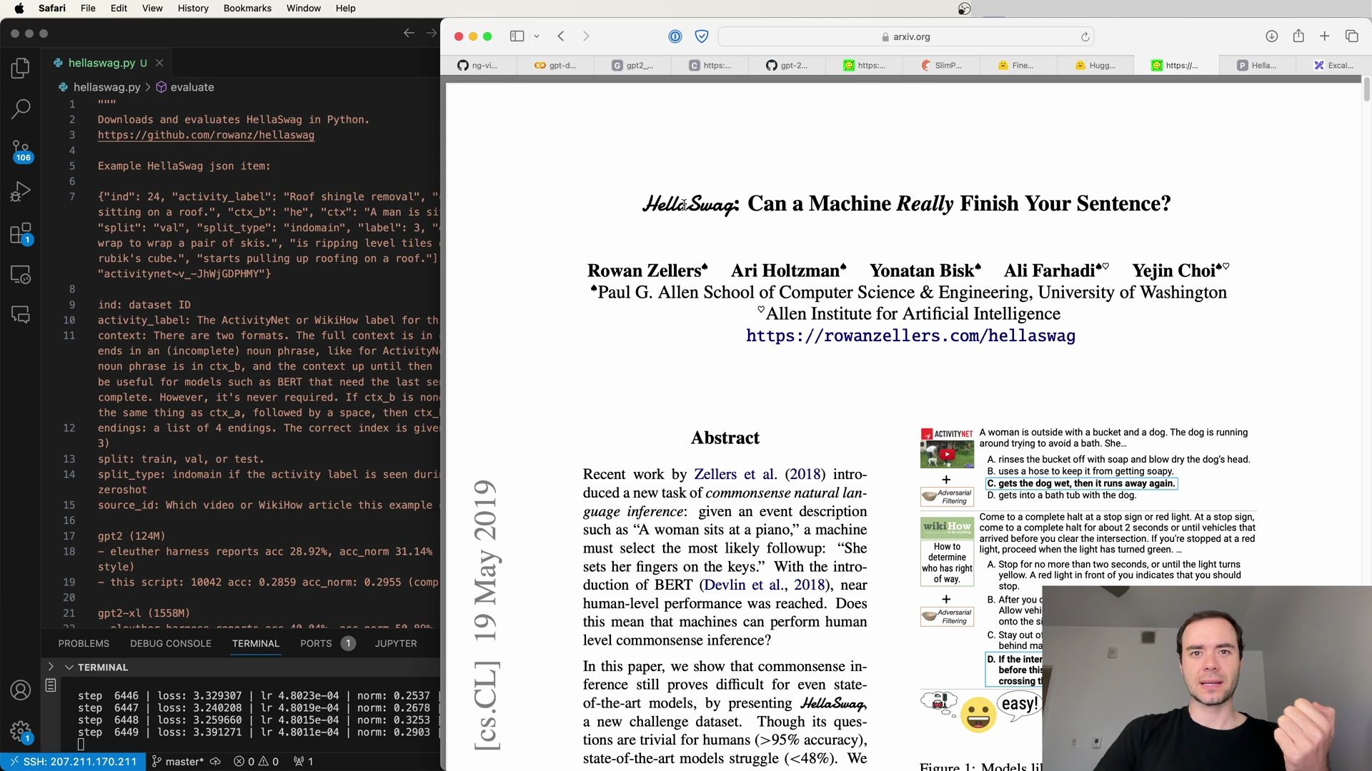
The task is to select the most natural continuation of the sentence. Let’s look at an example provided in the script:
A woman is outside with a bucket and a dog. The dog is running around trying to avoid a bath. She a) insists the bucket out was soap and blow dry the dog’s head, b) uses a hose to keep it from getting soapy, c) gets the dog wet and it runs away again, or d) gets into a bath tub with the dog.
The correct choice should be a plausible and natural continuation, showcasing the model’s ability to use commonsense reasoning.
Overview of HellaSwag and Adversarial Filtering
The HellaSwag dataset is a noteworthy contribution to the field of NLP due to its design that challenges even state-of-the-art models. Its creation involves a technique called Adversarial Filtering (AF), which is used to generate high-quality examples that are easy for humans but difficult for machines. The approach used for HellaSwag is detailed in the following extract:
- Title: HellaSwag: Can a Machine Really Finish Your Sentence?
- Authors: Rowan Zellers, Ari Holtzman, Yonatan Bisk, Ali Farhadi, Yejin Choi
- Institutions: Paul G. Allen School of Computer Science & Engineering, University of Washington; Allen Institute for Artificial Intelligence
- Abstract and Details: HellaSwag Dataset
The dataset consists of endings sourced from ActivityNet and WikiHow, with broad coverage across various domains such as computers, electronics, and home and garden, requiring a breadth of world knowledge to predict the most likely completions. Here’s an image that provides an example of the dataset:
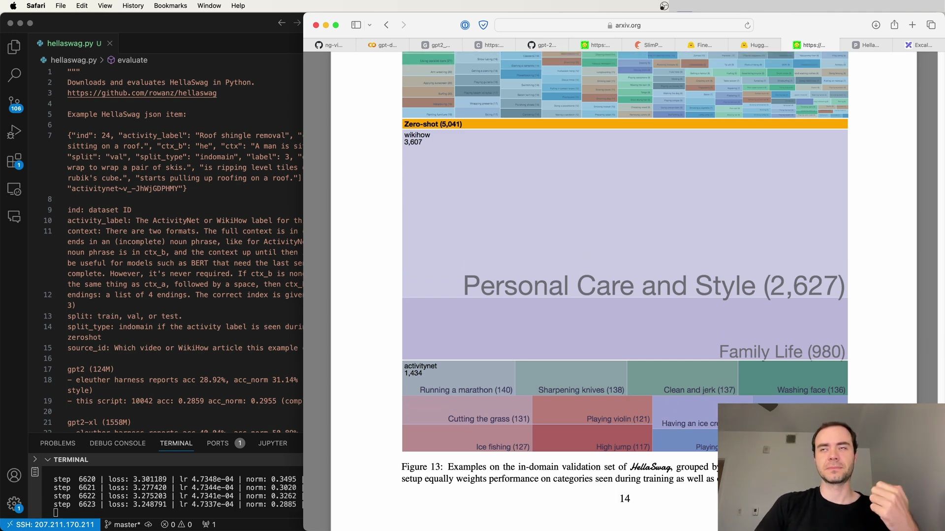
As the dataset challenges models with commonsense inference, it continues to be a valuable benchmark for evaluating language models.
Evaluating Models with HellaSwag
When it comes to evaluating language models, HellaSwag offers a smooth and early signal of performance improvement. This means that even small language models show incremental progress on the dataset, which is useful for tracking early stages of training.
Implementation of HellaSwag Evaluation
To evaluate our model using HellaSwag, we can use the evaluation script provided in the dataset’s repository. Here’s how to get started with evaluating HellaSwag in Python:
# Downloads and evaluates HellaSwag in Python.
# https://github.com/rowanz/hellaswag
# Code for evaluation would be here
This script makes it easy to download and evaluate our model’s performance on the HellaSwag dataset, providing us with an additional metric to assess the model’s ability for commonsense reasoning.
In conclusion, through meticulous documentation, adjusting tokenization lengths, handling validation loss in distributed training, and using the HellaSwag dataset for evaluation, we are refining our language model to better understand and generate natural language. The continuous improvement in these areas ensures that our model not only performs well on paper but also demonstrates practical understanding and reasoning skills.
HellaSwag Token Completion Methodology
To effectively evaluate language models like ours with HellaSwag, we need to understand that smaller models, unlike their larger counterparts, cannot handle multiple-choice questions in the traditional sense. They aren’t equipped to associate labels with multiple-choice options. Consequently, we need to present the data in a form they can process: token completion.
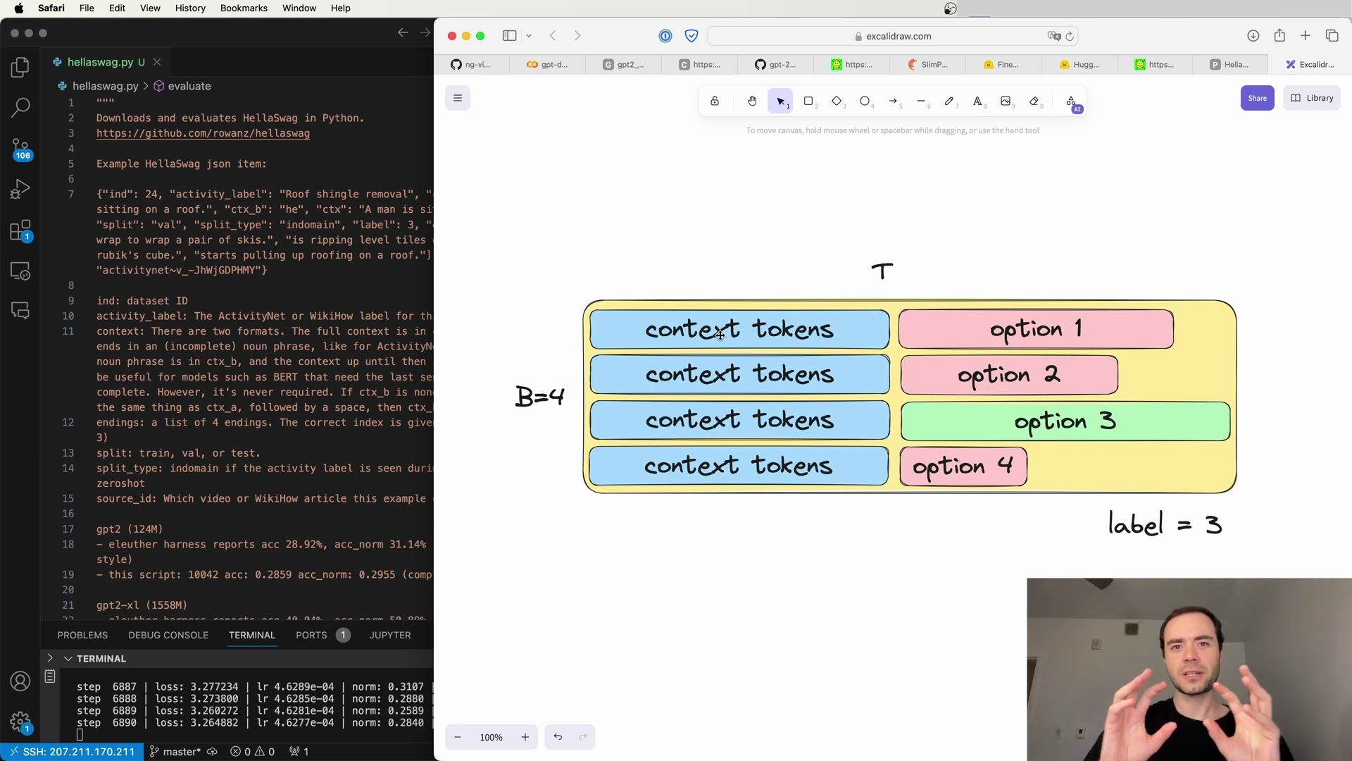
The evaluation approach involves constructing batches of four rows, each with T tokens, where T is determined by the length of the longest option to maintain consistency. The shared context, which is common to all four choices, is tokenized and distributed across the rows. Here’s an outline of the process:
- Construct a batch with four rows (options) and T tokens.
- Tokenize the shared context and distribute it across the rows.
- Include the four choice options, ensuring only one is correct.
- Use padding for options of varying lengths to maintain a consistent batch size (B x T).
- Implement a mask to identify active tokens, with zeros for padded areas.
The model will predict the most probable continuation by calculating the average probability for the tokenized options. It selects the option with the highest average probability as the correct choice.
Implementing HellaSwag Evaluation in Python
To integrate HellaSwag evaluation into our training pipeline, we can create a Python file, hella_swag.py, which includes:
- Functions to download and process the HellaSwag dataset.
- A rendering mechanism to convert examples into tokenized form.
- An evaluation function to load a language model and predict the correct continuation.
Here’s a glimpse into the Python implementation:
# hellaswag.py
import os
import json
import requests
import torch
import torch.nn as nn
from torch.nn import functional as F
from transformers import GPT2LMHeadModel
DATA_CACHE_DIR = os.path.join(os.path.dirname(__file__), 'cache_dir')
# Example of a function to download the dataset
def download(split):
# Code for downloading dataset
pass
# Function to render examples
def render_example(example):
# Code to tokenize context and choices
pass
# Function to evaluate the model
def evaluate_model(model_type, device):
# Code to load the model and predict continuations
pass
This implementation covers the evaluation of the HellaSwag dataset using the token completion style, where the model considers one option at a time. It is worth mentioning that other evaluation methods may use a multiple-choice format where the model sees all options simultaneously. However, this is generally easier and only feasible for larger models.
Tracking Model Performance on HellaSwag
To accurately assess our model’s performance, we track its accuracy on the HellaSwag validation set. Here are some statistics from different model sizes using both multiple-choice and completion styles:
- GPT-2 (124M) accuracy: 28.92% (multiple-choice), 28.59% (completion)
- GPT-2 XL (1558M) accuracy: 40.04% (multiple-choice), 38.42% (completion)
The validation set consists of 10,042 examples, offering a comprehensive benchmark for our evaluations.
Detailed Evaluation Process
The hella_swag.py file contains functions that iterate through the examples, rendering them for the model to evaluate. The evaluation process involves loading the model from Hugging Face, tokenizing the examples, and computing logits. Here’s a detailed look at the evaluation function:
# hellaswag.py
# ... (other code)
def evaluate_model(model_type, device):
model = GPT2LMHeadModel.from_pretrained(model_type)
model.to(device)
num_correct = 0
num_total = 0
for example in iterate_examples('val'):
tokens, mask, label = render_example(example)
tokens = tokens.to(device)
mask = mask.to(device)
logits = model(tokens).logits
# Calculate losses and average for completion region
# ... (loss computation code)
# Predict the option with the lowest loss
pred = logits.argmin().item()
num_total += 1
num_correct += int(pred == label)
accuracy = num_correct / num_total
print(f"Accuracy: {accuracy}")
In this evaluation routine, the model’s predictions are compared against the correct labels, and accuracy is calculated accordingly. It’s critical to ensure that the model is configured correctly and that the tokens and mask are accurately represented during evaluation.
Continuous Learning and Optimization
Our development process involves continuous learning and optimization. We adapt learning rates and optimization techniques to keep improving the model’s performance. Here’s an example of how we might adjust the learning rate during training:
# hellaswag.py
# ... (other code)
def get_lr(iteration, max_steps, warmup_steps, max_lr, min_lr):
# Linear warmup
if iteration < warmup_steps:
return max_lr * (iteration + 1) / warmup_steps
# Hold at max_lr before decay
if iteration > max_steps:
return min_lr
# Cosine decay to min_lr
decay_ratio = (iteration - warmup_steps) / (max_steps - warmup_steps)
coeff = 0.5 * (1.0 + math.cos(math.pi * decay_ratio))
return min_lr + coeff * (max_lr - min_lr)
# Example usage within training loop
optimizer = model.configure_optimizers(with_lr_schedule=True)
# ...
for step in range(max_steps):
lr = get_lr(step)
# ...
By using techniques like linear warmup and cosine decay, we fine-tune the learning rate to achieve better convergence and performance on tasks such as HellaSwag.
In summary, by meticulously crafting our evaluation process for the HellaSwag dataset, we enable our language model to demonstrate its ability in commonsense reasoning and context understanding. This, combined with our continuous optimization and learning rate adjustments, propels our model towards more accurate and natural language processing capabilities.
Cross-Entropy Loss in Model Evaluation
To assess our model’s capacity to predict the next token in a sequence, we employ cross-entropy loss as a critical measure. This loss function is pivotal in determining whether the model assigns the lowest or the highest probability to the correct token continuation.

The cross-entropy loss is computed over the set of possible token continuations, providing a quantitative basis for the model’s predictions. By focusing on the loss incurred when predicting the next token, we gain insight into the model’s token-level understanding and its predictive abilities.
Evaluating Model Predictions
The process of evaluating model predictions involves calculating the average loss for tokenized options and identifying the option with the lowest average loss. Let’s walk through the evaluation function in our hella_swag.py script:
# hellaswag.py
# evaluate
def evaluate(model_type, device):
data, mask, labels = render_example(example)
tokens = tokens.to(device)
mask = mask.to(device)
# get the logits
logits = model(tokens).logits
# a progressive loss at all positions
shift_logits = logits[..., :-1, 1:].contiguous()
flat_shift_logits = shift_logits.view(-1, shift_logits.size(-1))
shift_losses = F.cross_entropy(flat_shift_logits, flat_shift_tokens,
reduction='none')
shift_losses = shift_losses.view(tokens.size(0), -1)
# now get the average loss just for the completion region (where mask == 1), in each row
shift_mask = mask[..., 1:].contiguous() # we must shift mask, so we start at the last prompt token
masked_shift_losses = shift_losses * shift_mask
sum_loss = masked_shift_losses.sum(dim=1)
avg_loss = sum_loss / shift_mask.sum(dim=1)
# now we have a loss for each of the 4 completions
# the one with the lowest loss should be the most likely
pred = sum_loss.argmin().item()
pred_norm = avg_loss.argmin().item()
# accumulate stats
num_total += 1
num_correct += int(pred == label)
num_correct_norm += int(pred_norm == label)
print(f"Accuracy: {num_correct / num_total}")
print(f"Normalized Accuracy: {num_correct_norm / num_total}")
This function adjusts the logits to account for the shifted positions in the token sequences and calculates the loss considering the mask that indicates active tokens. It then averages the loss for the region of interest, where the mask equals 1, and determines the most likely completion.
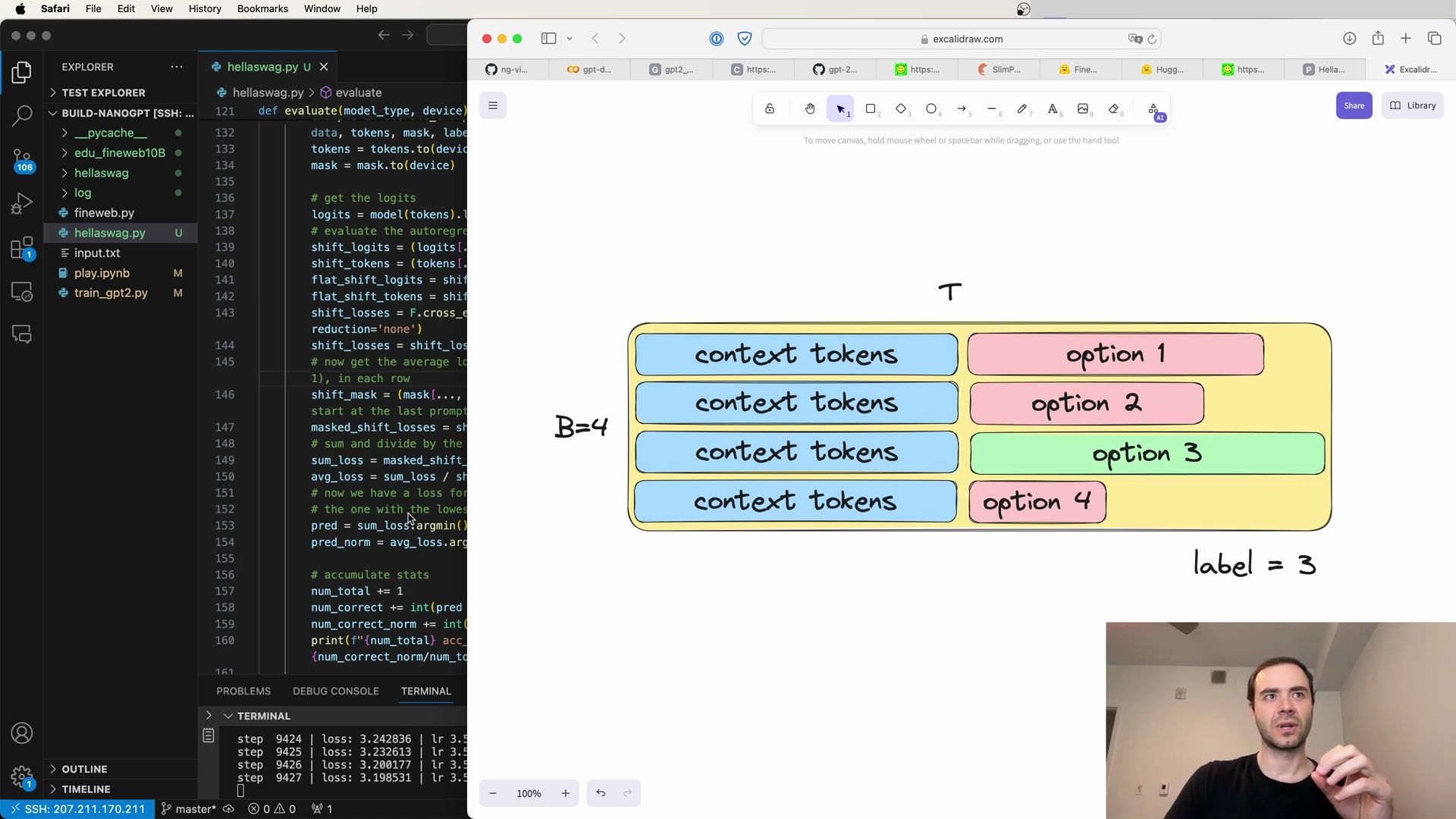
Performance Metrics
When evaluating the performance of GPT-2 models with our script, we observed the following:
- GPT-2 (124M) achieves an accuracy of 29.55%, modestly above the random chance of 25%.
- GPT-2 XL (1558M) reaches an accuracy of approximately 49%, demonstrating a significant improvement over its smaller counterpart.
These figures, however, still fall short of the state-of-the-art models, which currently exhibit accuracies around 95%, indicating there is substantial room for advancement.
ElutherAI Harness
ElutherAI Harness is a commonly used infrastructure for running evaluations on language models. It may yield slightly different numbers compared to our script, possibly due to variations in evaluation methodology, such as the use of multiple-choice versus token completion styles.
# hellaswag.py
# ... (code to set up the evaluation environment)
# Import necessary libraries
import os
import json
import requests
import itertools
from tqdm import tqdm
import torch
from torch.nn import functional as F
from transformers import GPT2LMHeadModel
# Set up the data cache directory
DATA_CACHE_DIR = os.path.join(os.path.dirname(__file__), 'cache_dir')
# ... (further code related to evaluation)
Integrating Periodic Evaluation
To monitor our model’s progress and performance over time, we must incorporate periodic evaluation into our main training script. This allows us to track improvements and determine when the model surpasses certain accuracy thresholds, such as the 29.55% region for GPT-2 (124M).
Changes to Training Script
Let’s review some of the modifications made to the train_gpt2.py script:
# train_gpt2.py M
# Adjustments to the training script
# Ensure the total batch size is divisible by the product of B, T, and ddp_world_size
assert total_batch_size % (B * H * T * ddp_world_size) == 0, "Ensure divisibility for batch size"
# Conditionally display messages on the master process
if master_process:
print(f'Calculated total batch size: {total_batch_size}')
print(f'Calculated gradient accumulation steps: {grad_accum_steps}')
# Prepare data loaders for training and validation
train_loader = DataLoaderLite(B=B, T=T, process_rank=ddp_rank, num_processes=ddp_world_size, split='train')
val_loader = DataLoaderLite(B=B, T=T, process_rank=ddp_rank, num_processes=ddp_world_size, split='val')
# Set higher precision for matrix operations
torch.set_float32_matmul_precision('high')
# Instantiate the model and move it to the device
model = GPT(GPTConfig(vocab_size=50304))
model.to(device)
# Disable torch.compile by default due to conflicts with HellaSwag evaluation
use_compile = False # torch.compile interferes with HellaSwag eval and Generation. TODO: fix
if use_compile:
model = torch.compile(model)
# Configure Distributed Data Parallel (DDP) if enabled
if ddp:
model = DDP(model, device_ids=[ddp_local_rank])
raw_model = model.module if ddp else model # always access the raw, unwrapped model
# Set learning rate parameters for training
max_lr = 6e-4
min_lr = max_lr * 0.1
warmup_steps = 715
max_steps = 19073
# Define a function to adjust learning rate based on the iteration
def get_lr(it):
# Linear warmup for warmup_iters steps
if it < warmup_steps:
return max_lr * it / warmup_steps
# Return minimum learning rate if iteration exceeds max_steps
if it > max_steps:
return min_lr
# Use cosine decay down to the minimum learning rate
decay_ratio = (it - warmup_steps) / (max_steps - warmup_steps)
assert 0 <= decay_ratio <= 1
# ... (training loop with logging of steps, loss, learning rate, etc.)
By incorporating these changes, we aim to optimize the training process and enable seamless integration of evaluation metrics like those used for the HellaSwag dataset. This strategic approach fosters a more refined and capable language model over time.
Debugging Training Issues
As we progress in fine-tuning our GPT-2 model, we sometimes encounter unexpected behaviors during training. One such issue arises when the evaluation code breaks during sampling, resulting in an early termination of the process. This anomaly could be attributed to various factors, including incorrect batch size calculations or inconsistencies in the model’s state during evaluation.
To ensure that the training process runs smoothly, it’s crucial to verify that the total batch size is a multiple of the product of batch size per step (B), sequence length (T), and the number of processes in a distributed data parallel setting (ddp_world_size). If this assertion fails, it indicates a potential misconfiguration that could disrupt the training workflow:
assert total_batch_size % (B * T * ddp_world_size) == 0, "Ensure divisibility for batch size"
Moreover, debug messages play a vital role in monitoring the state of the training process. These messages are conditionally displayed only on the master process to avoid cluttering the console with repeated outputs from multiple processes:
if master_process:
print(f'start: desired batch size: {total_batch_size}')
print(f'-> calculated gradient accumulation steps: {grad_accum_steps}')
Learning Rate Scheduling
Learning rate scheduling is a critical component of training deep learning models. A well-tuned learning rate schedule can lead to faster convergence and better model performance. In our train_gpt2.py script, we implement a cosine decay schedule for the learning rate. Starting at a maximum learning rate (max_lr), we slowly decay down to a minimum learning rate (min_lr) as training progresses:
# ... up here, we slowly decay down to the min learning rate
decay_ratio = (step - warmup_steps) / (max_steps - warmup_steps)
assert 0 <= decay_ratio <= 1
coeff = 0.5 * (1 + cos(math.pi * decay_ratio)) # coeff starts at 1 and goes to 0
return min_lr + coeff * (max_lr - min_lr)
The optimizer is then configured with this dynamic learning rate along with other hyperparameters such as weight decay:
optimizer = raw_model.configure_optimizers(weight_decay=0.1, learning_rate=6e-4, device=device)
Logging and Validation
To keep track of the model’s performance, we have established a logging mechanism that records the training and validation losses, as well as the HellaSwag accuracy, in a simple text file. The log file is first opened in write mode to clear its contents and then subsequently appended with new data:
# create the log directory we will write checkpoints to and log to
log_dir = 'training_runs'
os.makedirs(log_dir, exist_ok=True)
log_file = os.path.join(log_dir, 'log.txt')
with open(log_file, 'w') as f: # open for writing to clear the file
pass
During the training loop, we periodically evaluate the model’s validation loss to monitor its performance. This evaluation is carried out every 250 steps and on the last step of training:
for step in range(max_steps):
t0 = time.time()
last_step = (step == max_steps - 1)
# once in a while evaluate our validation loss
if step % 250 == 0 or last_step:
model.eval()
val_loader.reset()
with torch.no_grad():
val_loss_accum = 0.0
val_loss_steps = 20
for _ in range(val_loss_steps):
x, y = val_loader.next_batch()
x, y = x.to(device), y.to(device)
with torch.autocast(device=device, dtype=torch.bfloat16):
logits, loss = model(x, y)
loss = loss / val_loss_steps
Sampling from the Model
In addition to evaluating the validation loss, every 250th iteration also includes sampling from the model. Sampling allows us to observe the generative capabilities of our model and gain insights into the quality of the text it can produce. The following code demonstrates this process:
with torch.no_grad():
logits, loss = model(x[:, :-1]) # B, T, vocab_size
# take logits at the last position
logits = logits[:, -1, :] # B, vocab_size
probs = F.softmax(logits, dim=-1)
# book-keeping of logits
top_k_probs, top_k_indices = torch.topk(probs, 50, dim=-1)
# select a token from the top-k probabilities
# note: multinomial does not demand the input to sum to 1
ix = torch.multinomial(top_k_probs, 1, generator=sample_rng) # (B, 1)
# gather the corresponding indices
xcol = torch.gather(top_k_indices, -1, ix) # (B, 1)
# append to the sequence
xgen = torch.cat((xgen, xcol), dim=-1)
# print the generated text
for i in range(num_sequences):
tokens = xgen[i, :max_length].tolist()
decoded = enc.decode(tokens)
print(f'Generated text: {decoded}')
Optimization Step
The core of the training process is the optimization step, where the model is trained through backpropagation and the gradients are updated. The loss is scaled to account for gradient accumulation, which is important for larger models or when the available memory is limited:
# do one step of the optimization
model.train()
optimizer.zero_grad()
loss_accum = 0.0
for micro_step in range(grad_accum_steps):
x, y = train_loader.next_batch()
x, y = x.to(device), y.to(device)
with torch.autocast(device_type=device, dtype=torch.bfloat16):
logits, loss = model(x, y)
# we have to scale the loss to account for gradient accumulation,
# because the gradients just add on each successive backward().
# addition of gradients corresponds to a SUM in the objective, but
# instead of a SUM we want MEAN. Scale the loss here so it comes out right
loss = loss / grad_accum_steps
loss_accum += loss.detach()
if model.require_backward_grad_sync == (micro_step == grad_accum_steps - 1):
loss.backward()
if ddp:
dist.all_reduce(loss_accum, op=dist.ReduceOp.AVG)
norm = torch.nn.utils.clip_grad_norm_(model.parameters(), 1.0)
# determine and set the learning rate for this iteration
lr = get_lr(step)
The training loop outputs key metrics such as the current loss, learning rate, gradient norm, and tokens processed per second, allowing for real-time monitoring of the training process. This information is crucial for debugging and optimizing the model’s performance.
Fine-Tuning the Optimization Step
Improving the training process requires careful attention to the optimization step where the actual learning takes place. Let’s delve deeper into what happens during this crucial phase. In our train_gpt2.py script, the optimization is performed with gradient accumulation in mind. This approach is vital when dealing with large models or when GPU memory is limited. Here’s a more detailed look at the code:
# Perform one step of the optimization
model.train()
optimizer.zero_grad()
for micro_step in range(grad_accum_steps):
x, y = x.to(device), y.to(device)
with torch.autograd.set_detect_anomaly(True):
logits, loss = model(x, y)
# Scale the loss for gradient accumulation
loss = loss / grad_accum_steps
loss_accum += loss.detach()
if ddp:
# Ensure gradients are synchronized only on the last micro step
model.require_backward_grad_sync = (micro_step == grad_accum_steps - 1)
loss.backward()
if ddp:
# Average the accumulated loss across distributed processes
dist.all_reduce(loss_accum, op=dist.ReduceOp.AVG)
# Clip gradients to prevent exploding gradient problem
norm = torch.nn.utils.clip_grad_norm_(model.parameters(), 1.0)
# Update learning rate and optimizer for this step
lr = get_lr(step)
for param_group in optimizer.param_groups:
param_group['lr'] = lr
# Complete the optimization step
optimizer.step()
torch.cuda.synchronize() # Ensure the GPU has finished processing
t1 = time.time()
After each optimization step, we output key metrics to the terminal, providing insights into the model’s learning progress. Below is an example of how these metrics are reported:
step 10364 | loss: 3.149128 | lr 0.0331e-04 | norm: 0.2715 | dt: 420.08ms / tok
step 10365 | loss: 3.172654 | lr 0.0331e-04 | norm: 0.2728 | dt: 419.79ms / tok
step 10366 | loss: 3.196580 | lr 0.0331e-04 | norm: 0.2753 | dt: 420.99ms / tok
step 10367 | loss: 3.181015 | lr 0.0331e-04 | norm: 0.2694 | dt: 421.08ms / tok
HLSWag Evaluation
In addition to tracking the loss and other metrics, it’s essential to evaluate our model using a validation dataset. This evaluation helps us understand how well the model generalizes to new data. For the HellaSwag dataset, we follow a specific evaluation routine:
# Evaluate HellaSwag periodically
if (step % 250 == 0 or last_step) and (not use_compile):
num_correct = 0
num_total = 0
for _, example in enumerate(iterate_examples()):
# Skip examples not assigned to current process
if i % ddp_world_size != ddp_rank:
continue
# Process the example and obtain predictions
# ...
This distributed approach allows each GPU to handle a subset of the examples, which is crucial for efficient parallel processing. The model predicts the option with the lowest loss for each context, and the accuracy is determined by the number of correct predictions.
Tracking Correct Predictions
To track the number of correct predictions made by our model on the HellaSwag dataset, we employ the following steps:
# Initialize counters for correct predictions and total examples
num_correct = 0
num_total = 0
# Iterate over examples and update the counters
for i, example in enumerate(iterate_examples()):
# ...
# Check if the prediction is correct and update counters
if prediction == example['label']:
num_correct += 1
num_total += 1
Synchronizing Statistics Across Processes
When multiple processes collaborate on the evaluation, we need to synchronize their statistics. This process can be done by packaging the statistics into tensors and using distributed operations:
# Convert counters into tensors
num_correct_tensor = torch.tensor(num_correct).to(device)
num_total_tensor = torch.tensor(num_total).to(device)
# Sum the tensors across all processes
dist.all_reduce(num_correct_tensor, op=dist.ReduceOp.SUM)
dist.all_reduce(num_total_tensor, op=dist.ReduceOp.SUM)
# Convert tensors back to integers
num_correct = num_correct_tensor.item()
num_total = num_total_tensor.item()
# Master process logs the HellaSwag accuracy
if master_process:
hlswag_acc = num_correct / num_total
print(f"HellaSwag accuracy: {hlswag_acc}")
Logging and Sample Generation
Throughout training, we log important metrics and generate text samples to observe the model’s performance. After every 250 steps, and also on the last step, we log the validation loss and HellaSwag accuracy, and we generate text samples as follows:
if step % 250 == 0 or last_step:
# Switch to evaluation mode
model.eval()
# Generate text samples
num_return_sequences = 4
max_length = 32
tokens = enc.encode(some_input_text)
# Generate samples and log them
# ...
# Log directory setup
log_dir = 'log'
os.makedirs(log_dir, exist_ok=True)
log_file = os.path.join(log_dir, 'log.txt')
# Clear the log file and then append new data
with open(log_file, 'w') as f:
pass # Open for writing to clear the file
# Now append new log data
with open(log_file, 'a') as f:
f.write(f"step {step} | loss: {loss} | lr: {lr} | norm: {norm} | " \
f"dt: {dt}ms | tok/sec: {tokens_per_sec}\n")
The output includes a series of generated text samples that reflect the model’s current language generation abilities:
Hello, I'm a language model, so I'd like to use it to generate some kinds of output. Let's say there is a function for this.
Hello, I'm a language model, and I'm a developer for a lot of companies, but I'm writing a function in Haskell!
...
These samples give an immediate qualitative sense of what the model has learned and how it is performing on the task of generating coherent and contextually appropriate text.
Sample Generation Insights
As we continue to refine our language model, it’s fascinating to observe the kinds of outputs it generates at different stages of the training process. One notable observation is that the model starts using language that is more self-aware, acknowledging its identity as a language model. This progression suggests an increase in the model’s coherence and context awareness over time. For instance:
Hello, I'm a language model, so I'd like to use it to generate some kinds of output.
Hello, I'm a language model, and I'm a developer for a lot of companies, but I'm writing a function in Haskell!
These outputs demonstrate the model’s capability to construct sentences that are not only grammatically correct but also contextually relevant to its own identity.
Log Directory Setup
During the training of our GPT model, it’s crucial to maintain a directory where we can store checkpoints and logs. This is achieved through the following code snippet:
# Create the log directory we will write checkpoints to and log to
log_dir = "path_to_log_directory"
os.makedirs(log_dir, exist_ok=True)
This code ensures that the specified log directory exists or creates it if it does not. It’s an essential aspect of the training infrastructure, allowing us to keep track of the model’s progress and recover from any potential interruptions.
Visualization of Training Progress
To gain a deeper understanding of the training dynamics, we can visualize the training and validation losses as well as the HellaSwag evaluation scores. The following code snippet is used to parse and visualize the log file:
import numpy as np
import matplotlib.pyplot as plt
%matplotlib inline
# Parse the log file and extract metrics
# ...
# Visualize the training and validation losses
plt.plot(train_losses, label='Train Loss')
plt.plot(val_losses, label='Validation Loss')
plt.legend()
plt.xlabel('Steps')
plt.ylabel('Loss')
plt.title('Training vs. Validation Loss')
plt.show()
# Visualize the HellaSwag evaluation accuracy
plt.plot(hlswag_scores, label='HellaSwag Accuracy')
plt.legend()
plt.xlabel('Steps')
plt.ylabel('Accuracy')
plt.title('HellaSwag Evaluation Accuracy Over Time')
plt.show()
This visualization helps us identify any potential overfitting or underfitting and make necessary adjustments to the training process.
Model Configuration and Initialization
The GPT model is created with a specific configuration that includes the size of the vocabulary. The initialization of the model is as follows:
torch.set_float32_matmul_precision('high')
# Create model
model = GPT(GPTConfig(vocab_size=50304))
# Optionally initialize from a pretrained model
# model = GPT.from_pretrained('gpt2')
model.to(device)
This snippet sets the precision for matrix multiplication operations and initializes the model with a specified vocabulary size. Optionally, one can also load a pre-trained model to fine-tune it on a specific dataset.
Training Loop Adjustments
The training loop includes important parameters like learning rate schedule and gradient accumulation steps. An excerpt from the training loop is shown below:
max_lr = 6e-4
min_lr = max_lr * 0.1
warmup_steps = 715
max_steps = 119073 # Approximate steps for one epoch
# Define the learning rate schedule
def get_lr(it):
# Linear warmup
if it < warmup_steps:
return max_lr * (it + 1) / warmup_steps
# Cosine decay to min learning rate
decay_ratio = (it - warmup_steps) / (max_steps - warmup_steps)
return min_lr + (max_lr - min_lr) * (1 + np.cos(np.pi * decay_ratio)) / 2
# Training step
for step in range(max_steps):
optimizer.zero_grad()
# ...
This code configures a learning rate that linearly warms up to a maximum value and then decays following a cosine schedule, which is a common approach to stabilize training in deep learning models.
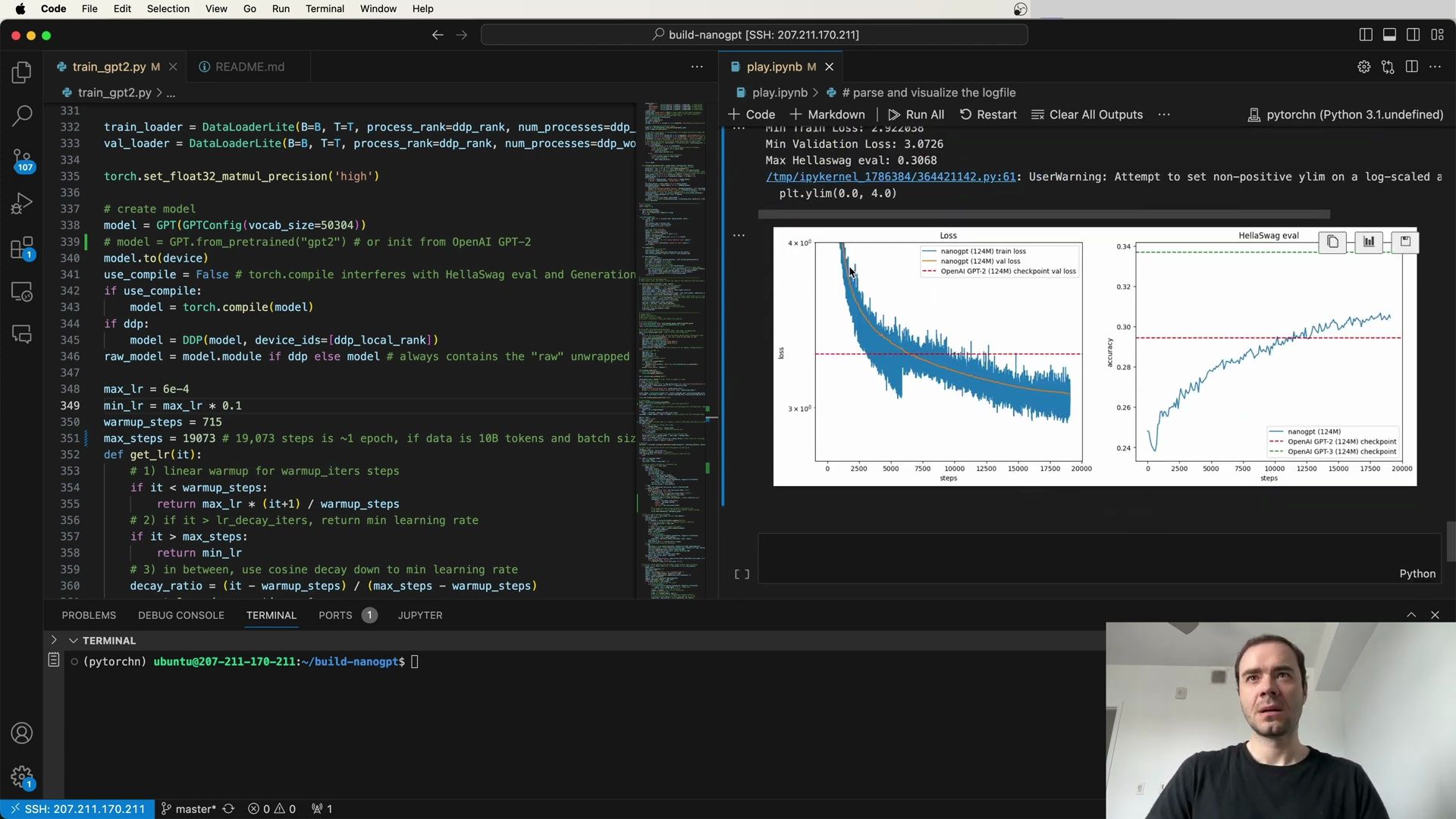
As we analyze the training progress graph, we observe the model’s loss decreasing over time, indicating effective learning. The minimum training loss, minimum validation loss, and maximum HellaSwag evaluation accuracy are key metrics that demonstrate the model’s performance.
HellaSwag Evaluation Outcomes
In the HellaSwag evaluation, we see that our model has surpassed the evaluation score of the OpenAI GPT-2 124M model, even though it was trained on significantly fewer tokens. This achievement suggests that our training regime or data quality might have contributed to the model’s efficiency.
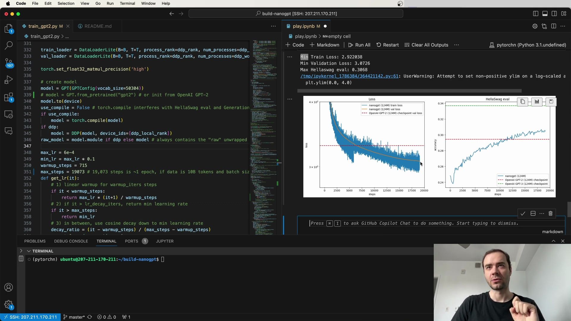
It’s important to note the caveat that our model was trained on a dataset with a different distribution than GPT-2’s original training data. The HellaSwag dataset serves as a standardized benchmark, providing us with a reliable measure of the model’s ability to generalize and understand context.
Considerations on Data Ordering
A final point to address is the potential impact of data shuffling or the lack thereof. Anomalies in the loss curve could be indicative of the training data not being properly shuffled, leading to periodic patterns that might affect the model’s learning dynamics. It’s essential to ensure that the data fed into the model during training is randomized to prevent any biases or artifacts from influencing the results.
In summary, the training process involves a complex interplay of factors including sample generation, log management, visualization, model configuration, learning rate scheduling, and evaluation benchmarks. By carefully monitoring and adjusting these elements, we can guide our language model toward improved performance and a better understanding of natural language.
Training Data Considerations
As we continue exploring the intricacies of training a language model like GPT-2, it’s important to reflect on some of the events that transpired post-recording. One crucial aspect is the quality of the training data. In the early days of language models, not as much care and attention went into dataset preparation. There’s been a shift towards better practices, such as duplication filtering and quality control, which likely contributes to our model’s improved performance.
The process of preparing a dataset for training a language model has evolved significantly. Here are some points to consider about data handling:
- Duplication Filtering: Ensuring that the dataset does not contain excessive duplicate entries, which can lead to overfitting.
- Quality Filtering: Removing low-quality data entries that might confuse the model or degrade its performance.
- Improved Datasets: It’s possible that our training dataset is of a higher quality per token compared to the original GPT-2 dataset, which could provide a performance boost.
DataLoaderLite Implementation
The DataLoaderLite class is instrumental in loading data efficiently for training. Here’s how it is initialized:
class DataLoaderLite:
def __init__(self, B, T, process_rank, num_processes, split):
self.B = B # Batch size
self.T = T # Sequence length
self.process_rank = process_rank
self.num_processes = num_processes
assert split in ['train', 'val']
# Get the shard filenames
data_root = 'edu_filtered/enwiki8B'
shards = os.listdir(data_root)
shards = [s for s in shards if split in s]
shards = sorted(shards)
shards = [os.path.join(data_root, s) for s in shards]
self.shards = shards
assert len(shards) > 0, "No shards found in the specified data_root."
This class handles the distribution of data across different processes, which is particularly useful for distributed training setups.
Data Ordering and Shuffling
Data ordering can significantly impact a model’s learning dynamics. In the initial setup, the model might not shuffle data properly, causing it to see documents in the same order during each epoch. This can introduce unwanted patterns and correlations that might bias the model.
To enhance the training process, consider implementing the following changes:
- Random Permutation: Shuffle documents within each shard before every epoch.
- Shard Shuffling: Randomize the order of the shards themselves to further reduce potential biases.
These changes can help in breaking down spurious correlations and improve the model’s ability to generalize from the training data.
Training Batch Size Configuration
Configuring the batch size appropriately is essential for efficient training. Here’s an example configuration in the train_gpt2.py script:
total_batch_size = 524288 # Total batch size in number of tokens
B = 64 # Micro batch size
T = 1024 # Sequence length
assert total_batch_size % (B * T * ddp_world_size) == 0, "Batch size configuration error."
The total_batch_size variable defines the size of the batch in tokens, which should be divisible by the product of micro batch size, sequence length, and the number of distributed data processing units.
Learning Efficiency Insights
Our model’s performance suggests that we are achieving a 10x improvement in learning efficiency compared to GPT-3, even though our model is trained on significantly fewer tokens. This efficiency can be attributed to several factors, including improved data quality and training practices. It’s a testament to the model’s ability to learn effectively from a well-curated dataset.
Considerations for Hyperparameters Adjustment
Hyperparameters play a pivotal role in model performance. For instance, the learning rate (max_lr) might be set conservatively based on GPT-3’s parameters. There is potential for increasing the learning rate to accelerate training without compromising the model’s learning capabilities. It’s encouraged to experiment with these hyperparameters to find the optimal settings for your specific training scenario.
Setting Up the Training Environment
The training environment’s setup can have a considerable impact on the model’s training process. The following script excerpt shows how to determine the device for training and set the seed for reproducibility:
device = 'cpu'
if torch.cuda.is_available():
device = 'cuda'
elif hasattr(torch.backends, 'mps') and torch.backends.mps.is_available():
device = 'mps'
print(f'Using device: {device}')
torch.manual_seed(1337)
if torch.cuda.is_available():
torch.cuda.manual_seed(1337)
# Further setup for data loading and model creation
This script checks for GPU or MPS (Apple Silicon) availability and sets the device accordingly, ensuring the model utilizes the best available hardware. It also sets a manual seed to make the training process deterministic.
Visualization of Extended Training Results
After an extended overnight training session, it’s instructive to review the updated results:
- Minimum Training Loss: 2.69377
- Minimum Validation Loss: 2.9478
- Maximum HellaSwag Evaluation Score: 0.3337
plt.ylim(0.0, 4.0)
# Plotting Loss and Evaluation Scores
plt.plot(train_losses, label='Train Loss')
plt.plot(val_losses, label='Validation Loss')
plt.plot(hellaswag_scores, label='HellaSwag Accuracy')
plt.legend()
plt.xlabel('Steps')
plt.ylabel('Metrics')
plt.title('Extended Training Results')
plt.show()
This graph demonstrates the model’s performance over an extended training period, capturing key metrics such as training loss, validation loss, and the HellaSwag evaluation accuracy. The improvements in these metrics indicate successful model training and optimization over time.

Sequence Length Adjustment for Model Training
When fine-tuning our training parameters to match or surpass the capabilities of larger models like GPT-3, we must consider the sequence length (T). GPT-3 utilizes a sequence length of 2048, which is twice that of 1024, a common setting for earlier models. Adjusting the sequence length directly affects the model’s ability to process longer dependencies in the text. To maintain the same number of tokens processed per iteration, we can modify our batch size (B) and sequence length (T) accordingly:
# Adjusting sequence length and batch size
B = 32 # New micro batch size
T = 2048 # New sequence length
This ensures that the model, with a sequence length equal to GPT-3, maintains a consistent number of tokens per step, keeping computational requirements in check.
Loss Metrics and Comparison with Other Models
In evaluating our model’s performance, we consider various metrics, including training and validation losses. Here, we highlight the minimum training loss, minimum validation loss, and maximum HellaSwag evaluation score achieved so far:
- Minimum Training Loss: 2.69377
- Minimum Validation Loss: 2.9478
- Maximum HellaSwag Evaluation Score: 0.3337
Comparing these results with other models like OpenAI’s GPT-2 and GPT-3, we can assert that our model’s performance is competitive, especially considering that GPT-2 and GPT-3 are very similar in their approach.
DataLoaderLite and Training Process
The DataLoaderLite class is crucial for efficient data loading during training. Here’s how we utilize it:
train_loader = DataLoaderLite(B=B, T=T, process_rank=ddp_rank, num_processes=ddp_world_size)
val_loader = DataLoaderLite(B=B, T=T, process_rank=ddp_rank, num_processes=ddp_world_size)
By optimizing the data loading process, we can ensure that the model is fed with consistent and efficient data streams, which is essential for stable and robust training.
Model Creation and Configuration
Creating and configuring the model is a fundamental step. The following snippet shows how we initialize the model with a specific vocabulary size and ensure it is correctly placed on the training device:
# Model initialization
model = GPT(GPTConfig(vocab_size=50304))
model.to(device)
use_compile = False # torch.compile interferes with evaluations
if use_compile:
model = torch.compile(model)
if ddp:
model = DDP(model, device_ids=[ddp_local_rank])
raw_model = model.module if ddp else model # always contains the 'raw' unwrapped model
This setup prepares the model for training while addressing potential issues, such as the interference of torch.compile with certain evaluations.
Sample Generation Insights
Examining the samples generated by the model can provide insights into its language understanding and generation capabilities. Here is a glimpse into the diversity and coherence of the output from our model:
rank 1 sample 0: Hello, I'm a language model, and I've been thinking a lot already...
rank 6 sample 1: Hello, I'm a language model, not programming any other language like Java.
rank 7 sample 2: Hello, I'm a language model, and I like to think it's the only language...
These samples suggest that the model has a coherent understanding of its identity as a language model and can produce a variety of contextually relevant sentences.
Validation Loss Evaluation
Calculating validation loss is a critical step in assessing model performance. We accumulate loss over multiple steps to get a more stable estimate:
val_loss_accum = 0.0
val_loss_steps = 20
for _ in range(val_loss_steps):
x, y = val_data.next()
x, y = x.to(device), y.to(device)
with torch.no_grad():
logits, loss = model(x, y)
loss = loss / val_loss_steps
val_loss_accum += loss.detach()
This process ensures that we get an accurate measure of the model’s performance on unseen data.
Master Process Validation Loss Reporting
When running distributed training, it’s important that only the master process reports the validation loss. Here’s how we handle this:
if ddp:
val_loss_accum = val_loss_accum / torch.distributed.ReduceOp.AVG
if master_process:
print(f"Validation Loss: {val_loss_accum}")
This snippet averages the loss across distributed processes and ensures that the master process outputs the final validation loss, maintaining clarity and avoiding redundant outputs.
Visualization of Training and Evaluation Metrics
Visualizing training progress and evaluation scores is essential for understanding model performance over time. Below is an example of a graph plotting training and validation losses, along with HellaSwag evaluation scores:
plt.ylim(0.0, 4.0)
plt.plot(train_losses, label='Train Loss')
plt.plot(val_losses, label='Validation Loss')
plt.plot(hellaSwag_scores, label='HellaSwag Accuracy')
plt.legend()
plt.xlabel('Steps')
plt.ylabel('Metrics')
plt.title('Training and Evaluation Metrics')
plt.show()
This visualization aids in monitoring the model’s progress and identifying areas for improvement.
Overall, our model shows promising signs of learning efficiency and capability, as demonstrated by the coherent sample outputs and competitive loss metrics. The careful tuning of training parameters, efficient data handling, and thorough evaluation practices contribute to the robustness and performance of the model.
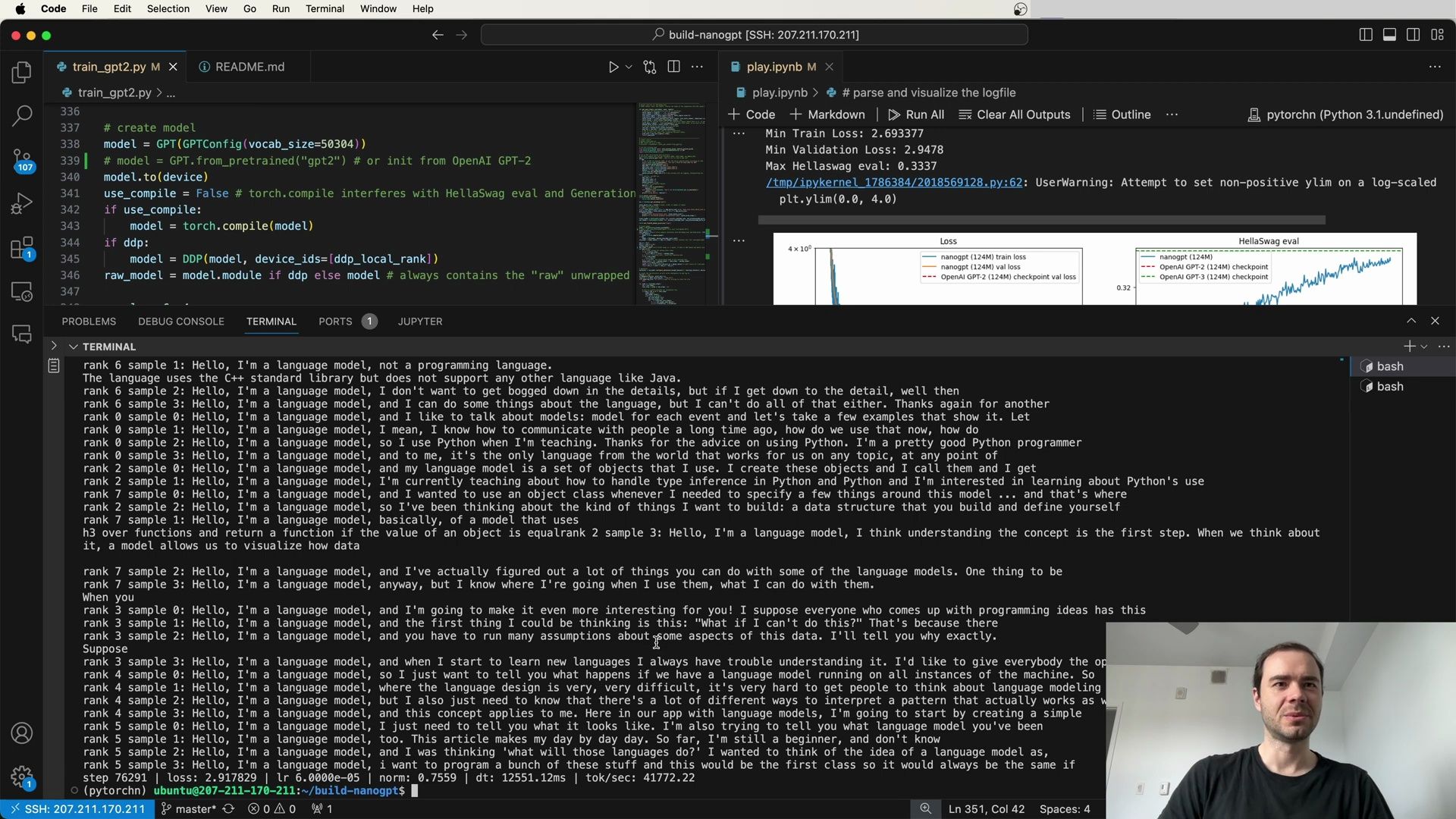
Checkpointing and State Management
In addition to logging the validation loss every 5000 steps, we’re implementing a checkpointing system. This is crucial for long training sessions, as it allows us to save the model’s state dictionary. Checkpointing is advantageous not only for potentially resuming the optimization process but also for later use in various evaluation settings. Here’s how we implement model checkpointing:
val_loss_accum = 0.0
val_loss_steps = 20
for _ in range(val_loss_steps):
x, y = val_loader.next_batch()
x, y = x.to(device), y.to(device)
with torch.no_grad():
logits, loss = model(x, y)
loss = loss / val_loss_steps
val_loss_accum += loss.detach()
if ddp:
dist.all_reduce(val_loss_accum, op=dist.ReduceOp.SUM)
if master_process:
print(f'validation loss: {val_loss_accum.item()}')
with open(log_file, 'a') as f:
f.write(f'{step} val {val_loss_accum.item()}\n')
if step > 0 and (step % 5000 == 0 or last_step):
# Model checkpointing code
checkpoint_path = os.path.join(log_dir, 'checkpoint_' + str(step))
checkpoint = {
'model': raw_model.state_dict(),
'config': raw_model.config,
'step': step,
'val_loss': val_loss_accum.item()
}
# Save additional states if needed
torch.save(checkpoint, checkpoint_path)
It’s important to note that the optimizer also has state that should be saved, particularly when using Adam, due to the additional momentum (m) and velocity (v) buffers. To fully resume training, one must also be mindful of saving and restoring random number generator (RNG) states.
Enhanced Evaluation with Luther
For a more thorough evaluation of the model, beyond just the HellaSwag dataset, we might consider utilizing the Luther Evaluation Harness. This tool allows for the assessment of language models across a variety of tasks, providing a more comprehensive understanding of the model’s capabilities. Here’s an example command using Luther for evaluation:
lm_eval --model hf \
--model_args pretrained=EleutherAI/gpt-j-6B \
--tasks hellaswag \
--device cuda:0 \
--batch_size 8
This command evaluates a model hosted on the HuggingFace Hub on the HellaSwag task using a CUDA-compatible GPU. Additional arguments can be passed to the model constructor, allowing for fine-tuned control over evaluation parameters.
Language Model Evaluation Harness
The Language Model Evaluation Harness provides a unified framework to test generative language models on a wide array of evaluation tasks. Key features include:
- Over 60 standard academic benchmarks
- Hundreds of subtasks and variants implemented
- Support for Jinja2 prompt design
- Config-based task creation and configuration
- Logging and usability changes
- New updates and features in the latest release
This framework ensures that language models can be evaluated in a consistent and thorough manner, providing a robust measure of their generalization capabilities across different contexts and benchmarks.
Comparison With Other Models
Evaluations are crucial for benchmarking our model against existing models such as OpenAI GPT-2. Here’s a quick comparison:
- Minimum Training Loss: 2.693377
- Minimum Validation Loss: 0.93478
- Maximum HellaSwag Evaluation Score: 0.3337
This comparison allows us to gauge the relative performance of our model. It is especially insightful when considering other tasks such as math, code, or processing different languages.
Pre-training and Fine-tuning
The journey of creating a language model begins with pre-training, where the model learns to predict the next token based on internet documents. Reproducing a GPT-2 (124M) model, for instance, has become much more accessible today and can be achieved in roughly an hour with modest costs. However, to engage in a conversation with the model, a fine-tuning step is required.
Fine-tuning, or supervised fine-tuning (SFT), involves swapping the dataset used in pre-training with one that is conversational, often structured in a user-assistant format. This step is relatively straightforward but essential for transforming a pre-trained model into a conversational agent like ChatGPT.
For those interested in the step-by-step building process of such models, the repository for nanoGPT provides a clear history of commits that show the gradual construction of the GPT model. This resource, coupled with an accompanying video lecture, offers a deep dive into the intricacies of language model development.
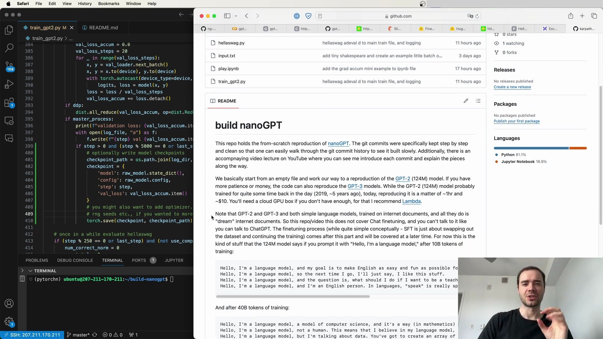
Conclusion
To summarize, the development of a language model involves a series of structured steps, from pre-training on large text corpora to fine-tuning for specific applications. The process is supported by tools and frameworks that assist in training, evaluation, and comparison with other models. Through checkpoints, we can preserve the state of the model, allowing for evaluation at different stages and providing a foundation for further fine-tuning tasks. With the help of comprehensive evaluation harnesses, we can ensure that our models are robust and perform well across various benchmarks.
Continuing Pre-training and Checkpointing
We now turn our attention to the continuation of the pre-training process. As we progress with training, it’s crucial to implement strategies that allow for efficient recovery and resumption. One method we employ is enhanced checkpointing. Here’s a more advanced checkpointing code that includes an anomaly detection feature to catch any unexpected gradients during backpropagation:
val_loss_accum = 0.0
val_loss_steps = 20
for _ in range(val_loss_steps):
x, y = val_loader.next()
x, y = x.to(device), y.to(device)
with torch.autograd.set_detect_anomaly(True):
logits, loss = model(x, y)
loss = loss / val_loss_steps
loss.backward()
val_loss_accum += loss.detach()
if ddp:
val_loss_accum = val_loss_accum / dist.ReduceOp.AVG
if master_process:
print(f'validation loss: {val_loss_accum.item()}')
In this snippet, we’ve integrated torch.autograd.set_detect_anomaly(True), which activates anomaly detection for the autograd engine. This can be helpful in identifying the exact operation that produced an “inf” or “NaN” during the backward pass.
Exploring Alternative Implementations
While we have been building towards the NanoGen GPT, it’s worth highlighting that there are other implementations out there. For instance, there’s a sibling repository to NanoGen GPT that offers a different approach to training the model. The following command line snippet illustrates how to run this alternative training script, showcasing various parameters such as batch size, sequence length, and learning rate:
python train_gpt2.py \
--input_val_bin 'dev/data/fineweb18/fineweb_val.bin' \
--val_loss_every 250 \
--sample_temperature 0 \
--write_tensor 0 \
--model_dir s \
--batch_size 64 \
--sequence_length 1024 \
--total_batch_size 524288 \
--dtype float16 \
--compile 1 \
--tensorscores 1 \
--flash 1 \
--num_iterations 18865 \
--weight_decay 0.1 \
--zero_stage 0 \
--learning_rate 0.0006 \
--warmup_iters 700 \
--learning_rate_decay_frac 0.0 \
--overfit_single_batch 0
This command specifies a directory for saving model checkpoints (--model_dir s), and enables options such as --write_tensor 0 and --compile 1, which refer to the process of writing tensors to disk and model compilation, respectively.
LN.C: A High-Performance C-CUDA Implementation
In a more recent project known as LN.C, we explore a C-CUDA implementation of GPT-2 or GPT-3. This implementation is written directly in C-CUDA and is expected to offer higher performance due to its direct optimization.
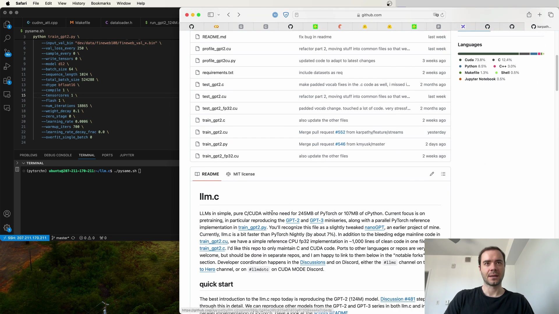
The LN.C repository acts as a reference to the aforementioned NanoGen GPT, implemented in PyTorch. The goal is to match the two implementations, with the expectation that the C-CUDA version will run faster due to being more directly optimized.
Training GPT2 in LN.C
For those interested in the finer details of the LN.C implementation, the train_gpt2.py script in the repository would look familiar, as it contains elements similar to those we’ve discussed in this lecture. Here’s a snippet of the command used to run the C-CUDA version of training:
python train_gpt2.py \
--input_val_bin 'dev/data/fineweb18/fineweb_val.bin' \
--val_loss_every 250 \
--sample_every 0 \
--write_tensors \
--model_dir s \
--batch_size 64 \
--sequence_length 1024 \
--total_batch_size 524288 \
--dtype fp16 \
--tensorcores 1 \
--flash 1 \
--num_iterations 18865 \
--weight_decay 0.1 \
--zero_stage 0 \
--learning_rate 0.0006 \
--warmup_iters 780 \
--learning_rate_decay_frac 0.0 \
--overfit_single_batch 0
This example showcases a typical training command with designated hyperparameters like learning rate, batch size, and the number of iterations, among others.
Side-by-Side Comparison
To illustrate the performance benefits of LN.C over the PyTorch implementation, we can run both side by side. By comparing the two, we can verify that they produce identical results, with LN.C demonstrating a faster execution time due to its optimized nature.
Observations and Performance
When observing the training process, we notice that LN.C compiles and allocates space swiftly, showcasing its efficiency. On the other hand, the PyTorch compilation process takes a bit longer, indicating the performance edge of the LN.C and BCC C-cuda compilation.
Conclusion
As we continue to refine and optimize our language models, it’s clear that the choice of implementation can have a significant impact on performance. LN.C stands as an example of how direct coding in C-CUDA can lead to faster training times and potentially more efficient models. With the right tools and approaches, such as advanced checkpointing and anomaly detection, we can achieve robust language models that are not only performant but also resilient in the face of long training sessions.
LN.C vs. PyTorch: Performance and Space Efficiency
When it comes to training GPT models, such as GPT-2 and GPT-3, it’s essential to consider the tools used for the task. While PyTorch is a versatile and widely-used neural network framework, LN.C, a C-CUDA implementation, is tailored specifically for training these types of models. Here are some key differences:
- PyTorch: Offers a general-purpose framework for various neural network models.
- LN.C: Provides a specialized and optimized approach for GPT-2 and GPT-3 models.
The LN.C implementation is not only very fast but also consumes less space. It is quicker to initialize and has a faster per-step execution time compared to PyTorch. This is particularly evident when looking at the token processing speed of both frameworks:
- LN.C: Approximately 223 thousand tokens per second.
- PyTorch: Approximately 185 thousand tokens per second.
This performance data shows that LN.C can be significantly faster than PyTorch, making it a competitive option for those focused on training GPT models.
Command-Line Training with PyTorch
For those who wish to train a GPT-2 model using PyTorch, the following command can be used to start the training process:
python train_gpt2.py \
--input_bin data/filename08b/filename08b_train.bin* \
--input_val_bin dev/data/filename08b/filename08b_val.bin* \
--v_loss_every 250
This command sets up a training run with the specified training and validation datasets, and configures the validation loss to be calculated every 250 steps.
LN.C: A Parallel Implementation
LN.C also offers a parallel implementation, which is an attractive option for those looking to experiment or seek faster performance. The implementation is designed to be straightforward and efficient, providing a good starting point for training on GPT models.
LLM.C: Simple and Pure C/CUDA Language Models
The LLM.C project takes a minimalist approach, offering language models in pure C/CUDA without the overhead of PyTorch or CPython. The project’s current focus is on pretraining and reproducing the GPT-2 and GPT-3 models. Here’s what you can expect from LLM.C:
- A slightly tweaked version of the earlier
nanoGPTproject. - A bit faster than PyTorch Nightly (by about 7%).
- Simple CPU fp32 implementation in roughly 1,000 lines of code.
Quick Start for LLM.C
If you are new to LLM.C, the best introduction is to reproduce the GPT-2 (124M) model. You can follow the discussion on the repository’s discussion boards for detailed steps. The repository also provides scripts to reproduce other models from the GPT-2 and GPT-3 series.
For those interested in single GPU training with fp32 precision and learning CUDA, the following steps outline how to run the GPU fp32 code:
pip install -r requirements.txt
python dev/data/tinyshakespeare.py
python train_gpt2.py
make train_gpt2fp32cu
./train_gpt2fp32cu
These commands will install the necessary requirements, prepare the data, and execute the training script for the fp32 implementation.
Training Insights and Tokenization
As we delve deeper into the training process of GPT models, we encounter various artifacts related to tokenization. Let’s explore some of the insights and configurations that can emerge during training:
class CausalSelfAttention(nn.Module):
def __init__(self, config):
super().__init__()
# key, query, value projections for all heads
self.c_attn = nn.Linear(config.n_embd, 3 * config.n_embd)
# output projection
self.c_proj = nn.Linear(config.n_embd, config.n_embd)
# regularization
self.n_head = config.n_head
self.n_embd = config.n_embd
# not really a 'bias', more of a mask, but following the OpenAI/HF naming
self.register_buffer("bias", ...)
This code block is a snippet from the CausalSelfAttention module within the train_gpt2.py script. It gives us a glimpse into how the self-attention mechanism is configured in the code, highlighting the projections for keys, queries, and values for all attention heads.
Consistency Between Implementations
One critical aspect of having multiple implementations is to ensure consistency in their performance. When aligning the steps and examining the output of both the LN.C and PyTorch models, it’s apparent that they produce identical results regarding loss and norm values. This consistency is crucial for confidence in training and model development.
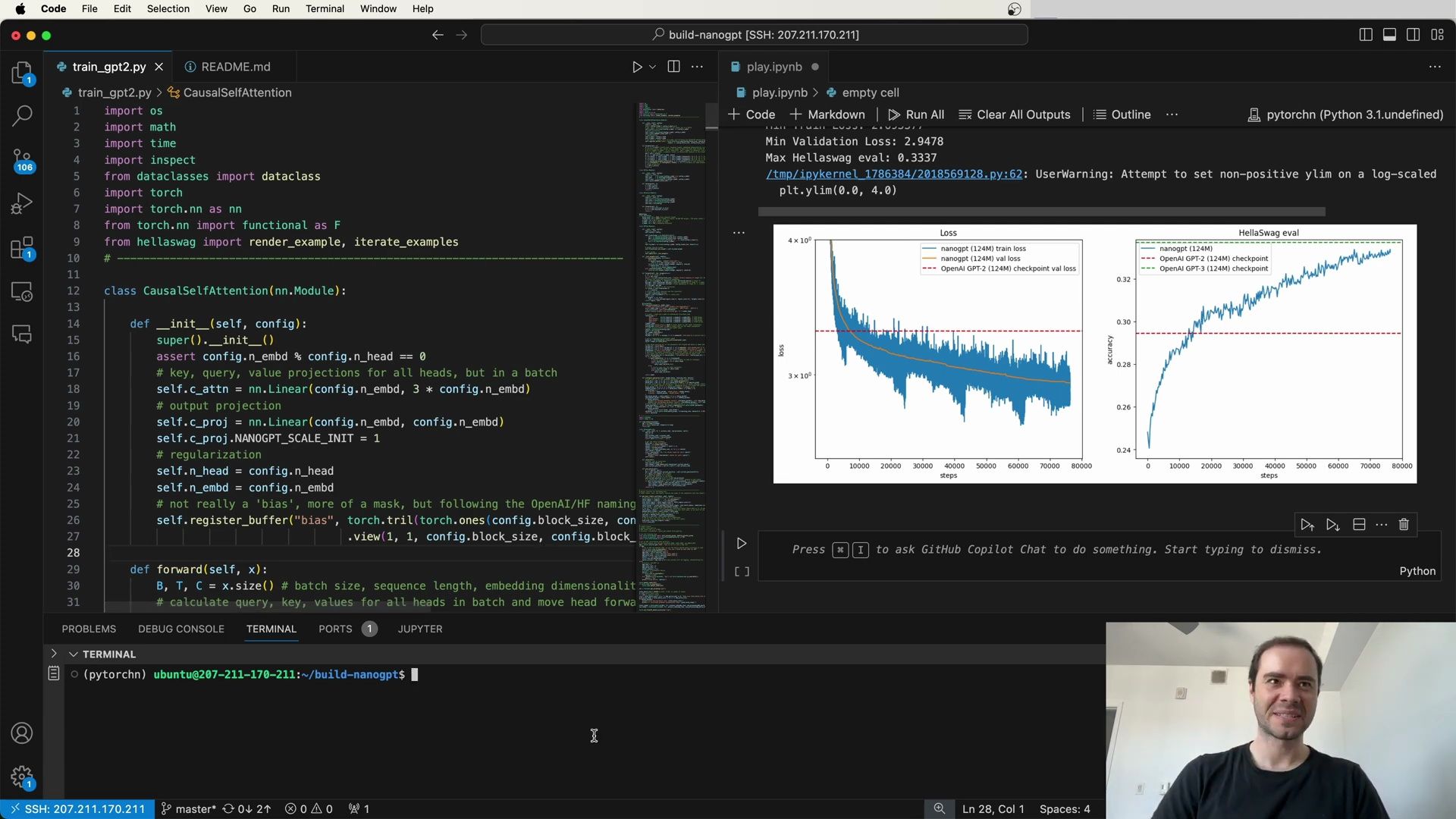
As shown in the image above, the side-by-side comparison of the training steps between LN.C and PyTorch demonstrates that both implementations yield the same training loss, norm, and learning rate, albeit with LN.C running at a faster pace.
Visualizing Model Training and Tokenization
The process of training a GPT model can be visualized to better understand the tokenization and learning dynamics. Here are a couple of insights from the images captured during training:
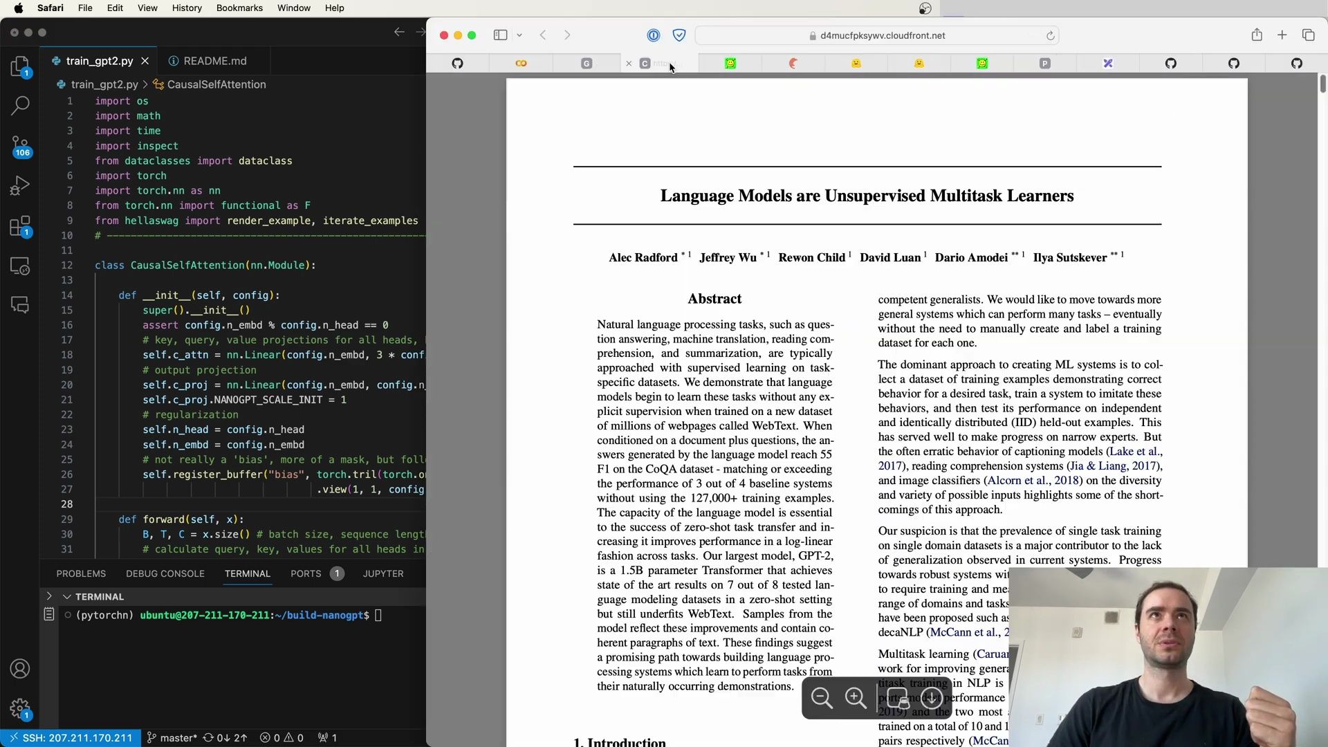
- The image provides a visual representation of the training dynamics, including the loss and evaluation metrics over time.
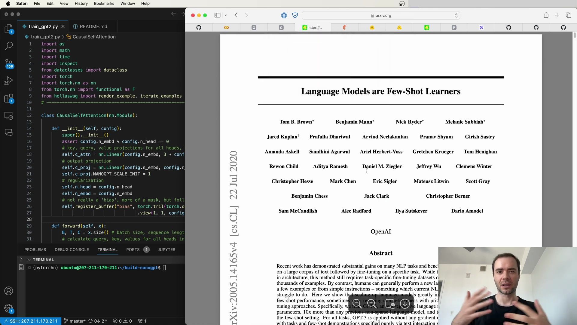
- This image displays code and tokenization elements that are part of the training script, giving us a deeper look into the inner workings of model training.
By piecing together these insights, we gain a comprehensive view of the training process, from the underlying code to the performance of the model during training.
Addressing Training Anomalies and Optimization
In the pursuit of training larger models like GPT-2 and GPT-3, one might encounter various issues that could impact the training dynamics, such as anomalies in loss curves. These issues often stem from data sampling strategies and other subtleties within the training process. It’s important to scrutinize these anomalies for a smoother training experience and better model performance.
For instance, fluctuations in the loss curve may indicate a need to adjust the batch data sampling or explore the possibility of overfitting. If you’re using PyTorch and encounter issues when trying to leverage torch.compile, it’s worth noting that it can sometimes break generation. Additionally, when reaching epoch boundaries, it’s advisable to permute your data to avoid introducing any biases or patterns that the model might latch onto inadvertently.
Building and Understanding nanoGPT
The nanoGPT repository serves as a from-scratch reproduction of the nanoGPT project. It is meticulously structured, with each git commit representing a step-by-step progression towards building the model. This approach, complemented by a YouTube lecture series, allows learners to follow along and understand each component of the model’s development.
Starting from a blank slate, the project culminates in a reproduction of the GPT-2 (124M) model. With patience and sufficient resources, one could even venture into reproducing GPT-3 models. Here’s a fascinating fact: while the GPT-2 (124M) model likely took substantial time to train back in 2019, now it can be reproduced in about an hour for approximately $10, provided you have access to a cloud GPU service like Lambda.
It’s essential to grasp that GPT-2 and GPT-3 are fundamentally simple language models trained on internet documents; they “dream” of internet documents. This repository does not delve into the finetuning process involved in creating models like ChatGPT. Finetuning, which conceptually entails swapping datasets and continuing training, will be covered separately.
Here’s an example of the output from the 124M model, trained on 10 billion tokens, when prompted with “Hello, I’m a language model”:
Hello, I'm a language model, and my goal is to make English as easy and fun as possible for you. Hello, I'm a language model, so the next time I go, I'll just say, I like this stuff.
Hello, I'm a language model, and the question is, what should I do if I want to be a teacher or a professor? Hello, I'm a language model, and I'm an English person. In languages, 'speak' is really sp...
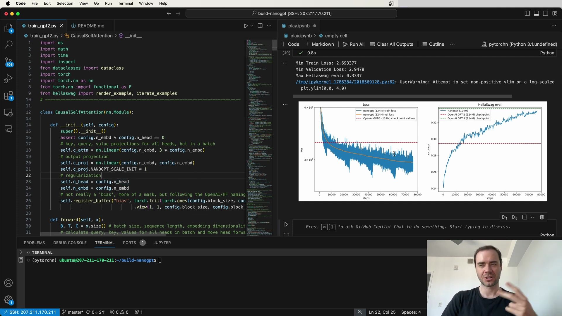
Community Engagement and Contributions
For those interested in discussing the intricacies of GPT model training or wishing to contribute to the development of such models, engaging with the community is invaluable. Questions, discussions, and contributions can be directed to forums like GitHub’s discussion boards, issues, and pull requests. This collaborative approach fosters a comprehensive understanding and facilitates collective advancement in the field.
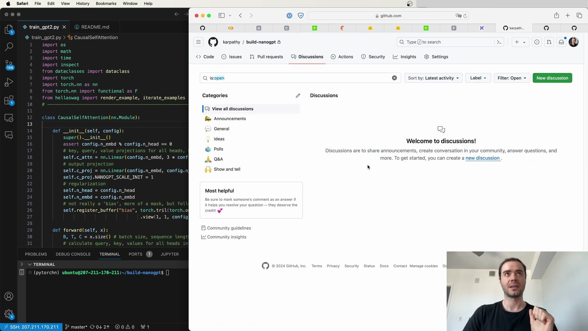
Furthermore, community spaces like Discord servers provide a place for real-time interaction with peers who share a common interest in language model training and implementation.
Causal Self-Attention in GPT-2 Training
The train_gpt2.py script includes a critical component known as the CausalSelfAttention module, which is at the heart of the GPT-2 model’s ability to generate coherent text by considering the context of each token. The Python code for this module is outlined below, highlighting the key, query, and value projections for all heads, as well as the output projection and the unique way bias is handled as a mask in this implementation.
import os
import math
import time
import inspect
from dataclasses import dataclass
import torch
import torch.nn as nn
from torch.nn import functional as F
from hellaswag import render_example, iterate_examples
class CausalSelfAttention(nn.Module):
def __init__(self, config):
super().__init__()
assert config.n_embd % config.n_head == 0
# key, query, value projections for all heads
self.c_attn = nn.Linear(config.n_embd, 3 * config.n_embd)
# output projection
self.c_proj = nn.Linear(config.n_embd, config.n_embd)
self.c_proj.NANOGPT_SAFE = True
# regularization
self.n_head = config.n_head
self.n_embd = config.n_embd
# not really a 'bias', more of a mask, but following the naming convention
self.register_buffer("bias", ...)
Reflecting on Progress and Future Directions
As we reach certain milestones in our journey of understanding and building language models, it’s beneficial to reflect on the progress made and consider the path forward. The training and implementation of GPT models are complex but rewarding endeavors that continue to evolve with advancements in the field.
As the community delves deeper into fine-tuning, model scaling, and optimization, there will always be new challenges and discoveries. The collective efforts of researchers, developers, and enthusiasts contribute significantly to the ongoing exploration of language models’ potential.
In conclusion, here are some training insights and benchmarks based on the nanoGPT project:
- Minimum Training Loss: 2.693377
- Minimum Validation Loss: 2.9478
- Maximum Hellaswag Evaluation: 0.3337
It’s important to note that these metrics are indicative of the model’s performance on specific tasks and datasets, and they provide a foundation for comparison with other models and checkpoints.
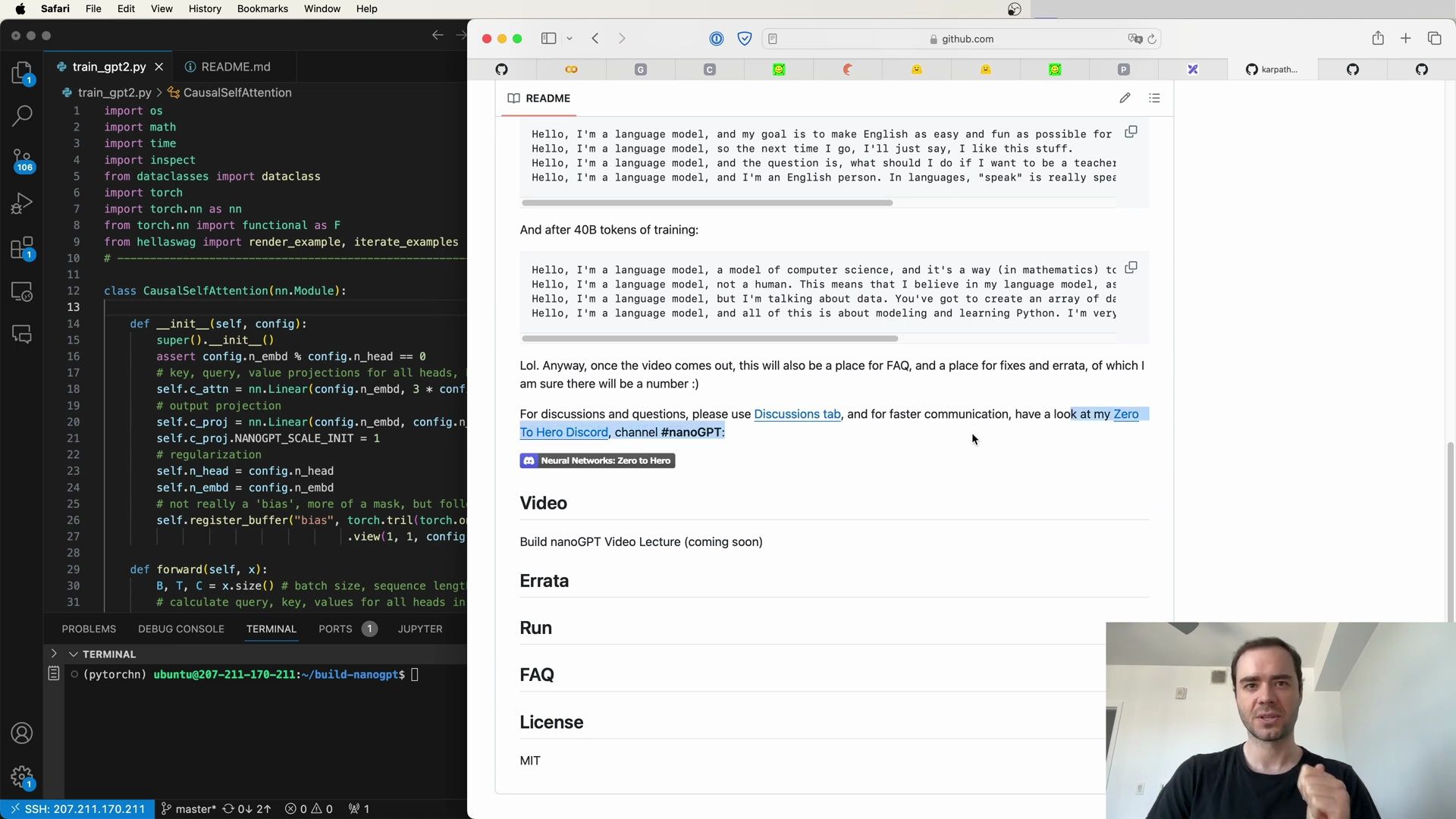
As we continue to explore and build upon these models, the ultimate goal remains to push the boundaries of what’s possible with language understanding and generation.
By meticulously configuring and observing the training process, from data handling to learning rate scheduling, and through continuous evaluation using benchmarks like HellaSwag, we can guide our language models toward improved performance and a better understanding of natural language. The insights gained from this deep dive into advanced model configuration and training optimization are instrumental in pushing the boundaries of language modeling and achieving state-of-the-art results.